
 buy artwork
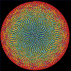
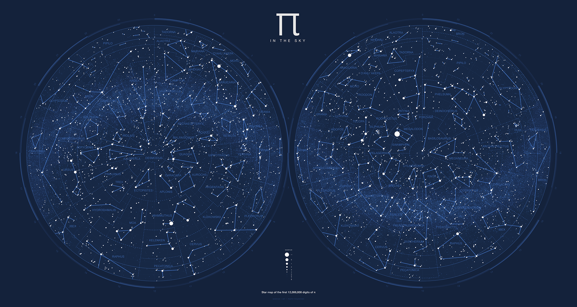
`\pi` Day 2017 Art Posters - Star charts and extinct animals and plants


On March 14th celebrate `\pi` Day. Hug `\pi`—find a way to do it.
For those who favour `\tau=2\pi` will have to postpone celebrations until July 26th. That's what you get for thinking that `\pi` is wrong. I sympathize with this position and have `\tau` day art too!
If you're not into details, you may opt to party on July 22nd, which is `\pi` approximation day (`\pi` ≈ 22/7). It's 20% more accurate that the official `\pi` day!
Finally, if you believe that `\pi = 3`, you should read why `\pi` is not equal to 3.

Caelum non animum mutant qui trans mare currunt.
—Horace
This year: creatures that don't exist, but once did, in the skies.
This year's `\pi` day song is Exploration by Karminsky Experience Inc. Why? Because "you never know what you'll find on an exploration".


create myths and contribute!
Want to contribute to the mythology behind the constellations in the `\pi` in the sky? Many already have a story, but others still need one. Please submit your stories!
Here I make available all the files you need to reconstruct the chart. All files are plain text and designed to be easily parsable.
 buy artwork
For the simplest chart, you'll need the star catalogue which already provides the longitude and latitude coordinates for each star. It'll be up to you to choose and calculate a projection.
You can then layer constellations, which are defined by a list of edges. If you like, you can draw boundaries around each constellation, which are also provided.
Star-to-constellation mapping is also given, which allows you to create labels for the stars within each constellation based on relative brightness.
Finally, you can get the species details for each constellation, including the Latin name of the species, Wikipedia URL and (for many) the mythology of the constellation.
star catalogue
The star catalog generated from the first 12 million digits of `\pi`.
DOWNLOAD

#   idx       digits   name      x      y      z     long      lat      dist  mabs  mapp
      0 314159265358      a  -1859    926     35  145.339   38.384  2077.157  3.00 14.59
      1 979323846264      b   4793  -2616    126  -38.404  -39.555  5461.884 -1.00 12.69
      2 338327950288      c  -1617  -2205   -472 -110.162   32.164  2774.797  3.00 15.22
      3 419716939937      d   -803  -3307    493 -105.489    3.655  3438.620  2.00 14.68
...
 999996 601538500580  cexhk   1015  -1150   -442  -48.144  -14.704  1596.273 -5.00  6.02
 999997 420478142596  cexhl   -796   2814   -241   97.939   14.471  2934.330  1.00 13.34
 999998 278256213419  cexhm  -2218    621   -159  156.900   46.719  2308.776  4.00 15.82
 999999 453839371943  cexhn   -462  -1063   -306  -95.924   26.937  1198.770 -2.00  8.39
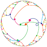
constellation definitions
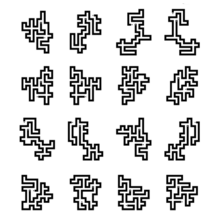
Constellations were manually defined. Each constellation has a name and abbreviation (first 3 characters unless longer is required to uniquely specify it). Shown next is the number of stars used to define the constellation and their names, as appear in the star catalogue file above. Next is the number of edges and the star pairs that define the edges of the constellation. The edges are not in any particular order and have no direction. Any spaces in names are encoded with _.
DOWNLOAD

# idx n_stars n_edges name abbrev stars edges
 ...
 2  3  3                   alaotra     ala blts,btosf,cbkbw btosf-cbkbw,blts-btosf,blts-cbkbw
 3  4  4                 alloperla     all ghyr,pwkn,ssrx,ugwt pwkn-ssrx,pwkn-ghyr,ugwt-pwkn,ssrx-ghyr
 4  2  1                   aplonis     apl cbocd,rllm rllm-cbocd
 ...
You can use this file to quickly search for certain shapes. For example, triangular constellations are those that have 3 stars and 3 edges.
> grep " 3  3" constellations.def.txt
 2  3  3                   alaotra     ala blts,btosf,cbkbw btosf-cbkbw,blts-btosf,blts-cbkbw
16  3  3                   camptor    camp benxf,bqvh,bwqed bqvh-benxf,bwqed-bqvh,bwqed-benxf
26  3  3                  desmodus     des bfnqu,mork,zwzy bfnqu-mork,zwzy-bfnqu,zwzy-mork
27  3  3                ectopistes     ect bopmt,cbquf,wmnw cbquf-bopmt,wmnw-cbquf,wmnw-bopmt
30  3  3                    hoopoe     hoo bpsop,bvmjh,tryh tryh-bvmjh,bpsop-tryh,bpsop-bvmjh
31  3  3                      huia     hui ccteo,xbvq,yqet xbvq-yqet,ccteo-xbvq,ccteo-yqet
39  3  3               malpaisomys     mal bucqd,likq,nqn nqn-bucqd,likq-nqn,likq-bucqd
41  3  3                   mariana     mar gmps,jydb,pcjx pcjx-gmps,jydb-pcjx,jydb-gmps
49  3  3          palaeoaldrovanda     pal bedae,oife,saz bedae-saz,oife-bedae,oife-saz
63  3  3                    rhynia     rhy bpviv,cenuk,hivz bpviv-hivz,cenuk-bpviv,cenuk-hivz
65  3  3                  silphium     sil bjesg,bmquw,bpxia bmquw-bpxia,bjesg-bmquw,bjesg-bpxia
69  3  3                   tadorna     tad bukqe,cbtrx,epdx cbtrx-epdx,bukqe-cbtrx,bukqe-epdx
72  3  3                 traversia     tra fcnw,fywb,puib fywb-fcnw,puib-fywb,puib-fcnw
80  3  3                  yersinia     yer colq,ibls,zgvy ibls-zgvy,colq-ibls,colq-zgvy
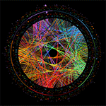
constellation boundaries
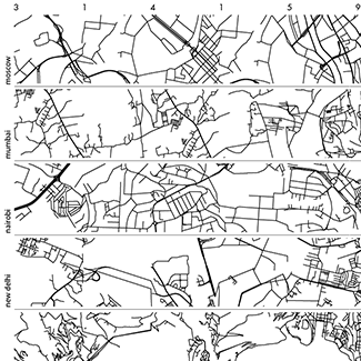
The boundaries were manually defined. Shown here, for each constellation, is the constellation's area, perimeter center and boundary `(x,y)` pairs, delimited by : and represent a closed polygon that encloses the constellation's stars.
All values are longitude and latitude. The three constellations listed below are ones with smallest area.
DOWNLOAD

# abbrev area perimeter centroid_xy boundary_xy_pairs

...
com 74.83 34.96 -102.50,26.25 -100.00,30.00:-102.50,30.00:-105.00,30.00:-107.50,30.00:-107.50,27.50:
			      -107.50,25.00:-107.50,22.51:-105.00,22.51:-102.50,22.51:-100.00,22.51:
			      -97.51,22.51:-97.51,25.00:-97.51,27.50:-97.51,30.00:-100.00,30.00
pal 50.02 30.00 3.43,-40.93 5.00,-37.49:2.50,-37.49:0.00,-37.49:0.00,-40.00:0.00,-42.50:0.00,-45.00:
			    2.50,-45.00:5.00,-45.00:5.00,-42.50:7.49,-42.50:7.49,-40.00:7.49,-37.49:5.00,-37.49
sil 37.57 25.02 115.00,-51.25 115.00,-47.50:112.49,-47.50:112.49,-50.00:112.49,-52.49:112.49,-55.00:
    	  		      115.00,-55.00:117.50,-55.00:117.50,-52.49:117.50,-50.00:117.50,-47.50:115.00,-47.50
The boundary polygons abut but do not overlap and they cover the entire sky. There is one polygon per consetllation. The total area of all constellations is `360 × 180 = 36800`.
constellation star membership
This is a list of all the stars on the chart and their constellation membership. A star is considered to be in a constellation if it falls within the constellation boundary.
The `i` and `j` indexes give the relative brightness of the star on the map and in the constellation, respectively. If a star is used to define the constellation edges it gets a + otherwise -.
DOWNLOAD

# abbreviation star i j mapp on_edge?
     aep bkawv     35     0   1.34 +
     aep   gql     65     1   1.63 +
     aep cavix     72     2   1.71 +
     aep bqxvm    137     3   2.25 +
     aep  tjow    158     4   2.31 +
     aep beelq    176     5   2.39 +
...
     yer  jjlj  39365   412   7.24 -
     yer bgswm  39464   413   7.24 -
     yer  ittu  39546   414   7.24 -
     yer  wakp  39556   415   7.24 -
     yer bedks  39667   416   7.25 -
     yer  gxzo  39817   417   7.25 -
To lookup the 10 brightest stars, sort on the i index. Here we see that megal (Megalodon) has the brightest star in the sky, jkxo with apparent magnitude `-2.05`. The next two brighest stars are in mam (Mammuthus) and ara (Araucaria).
> cat constellations.stars.txt | sort -n +2 -3 | head -10
   megal  jkxo      0     0  -2.05 +
     mam btsqy      1     0  -0.73 +
     ara ccijs      2     0  -0.38 +
     rap btaum      3     0   0.26 +
     urs bxlss      4     0   0.26 +
     tec bgrdk      5     0   0.43 +
     cop  itwr      6     0   0.45 +
     ara  mrvq      7     1   0.54 +
     phe  loju      8     0   0.54 +
     mam bhlbw      9     1   0.55 +
To get a list of the brightest star in each constellation, just search for " 0 ". Below I show this list sorted by brightness.
> cat constellations.stars.txt | grep " 0 "| sort -n +4 -5
   megal  jkxo      0     0  -2.05 +
     mam btsqy      1     0  -0.73 +
     ara ccijs      2     0  -0.38 +
     rap btaum      3     0   0.26 +
     urs bxlss      4     0   0.26 +
     tec bgrdk      5     0   0.43 +
     cop  itwr      6     0   0.45 +
     phe  loju      8     0   0.54 +
     kel bnhwx     11     0   0.59 +
     spe  rtep     13     0   0.71 +
     ...
     nes  vxou    299     0   2.80 -
     aur bmjvf    307     0   2.81 +
     tra  puib    318     0   2.83 +
     pip  cecq    358     0   2.91 +
     pal  oife    389     0   2.97 +
     swa   gvr    463     0   3.12 +
     hui ccteo    485     0   3.17 +
     ple bzqur    506     0   3.20 +
     com  ygrn    875     0   3.64 +
     car  yjkn    933     0   3.68 +
For example, tec (Tecopa) has bgrdk as its brightest star, which is 6th brightest in the sky with an apparent magnitude of 0.43.
The constellation whose brightest star is dimmest of all first brightest stars is car (Caracara). Its brightest star is yjkn which is 934th brightest in the sky with an apparent magnitude of 3.68.
To get the number of stars in each constellation, just add the number of times the constellation abbreviation appears. Bron has the most stars of any constellation, more than twice as many as the next one, archaeo (Archaeopteryx). Both car (Caracara) and por (Porzana) have only 7 stars each, the fewest of all constellations.
   5230 bro
   2287 archaeo
   2205 thy
   2155 kim
   1838 archaea
   1789 came
   1768 ard
...
     20 megal
     19 swa
     17 mar
     12 rhy
      8 sil
      7 por
      7 car
constellation names, stories and links
The constellations are in no particular order in this file.
DOWNLOAD

# constellation name
# hemisphere (n north, s south, b both)
# common name
# Latin name
# extinction date
# URL
# optional story

aplonis
n
mysterious bird of Ulieta
Aplonis ulietensis
1774-1850
https://en.wikipedia.org/wiki/Raiatea_starling

desmodus
n
Giant Vampire Bat
Desmodus draculae
Pleistocene or early Holocene
https://www.thoughtco.com/recently-extinct-shrews-bats-and-rodents-1092147
It is thought that each night Desmodus flies up against the dome of the sky, looking for a way to escape.

...
Beyond Belief Campaign BRCA Art
Fuelled by philanthropy, findings into the workings of BRCA1 and BRCA2 genes have led to groundbreaking research and lifesaving innovations to care for families facing cancer.
This set of 100 one-of-a-kind prints explore the structure of these genes. Each artwork is unique — if you put them all together, you get the full sequence of the BRCA1 and BRCA2 proteins.

Propensity score weighting
The needs of the many outweigh the needs of the few. —Mr. Spock (Star Trek II)
This month, we explore a related and powerful technique to address bias: propensity score weighting (PSW), which applies weights to each subject instead of matching (or discarding) them.
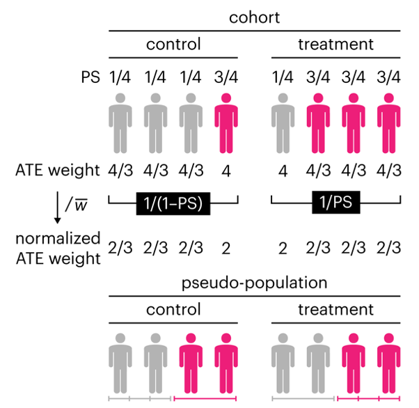
Kurz, C.F., Krzywinski, M. & Altman, N. (2025) Points of significance: Propensity score weighting. Nat. Methods 22:1–3.
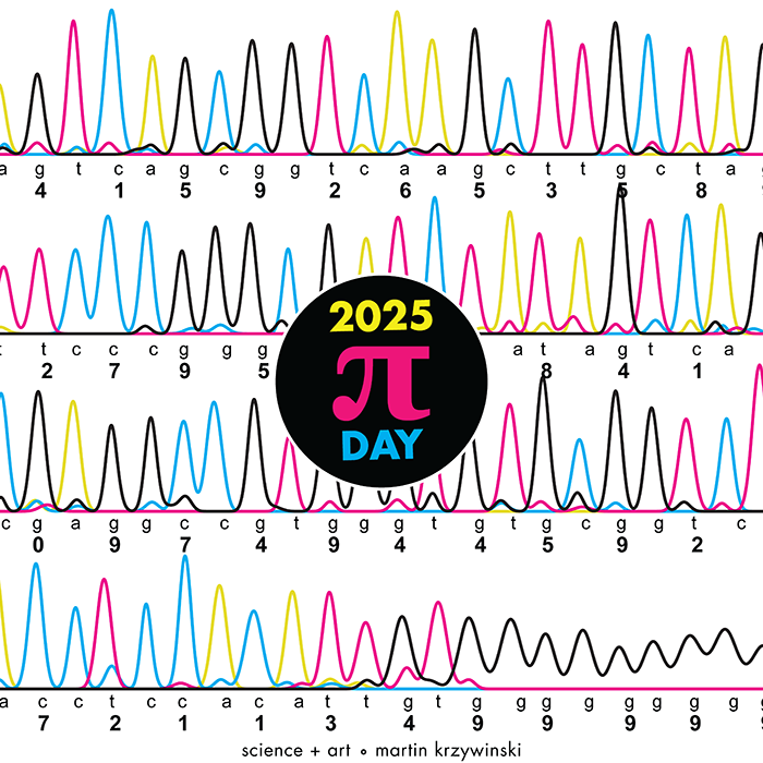
Happy 2025 π Day—
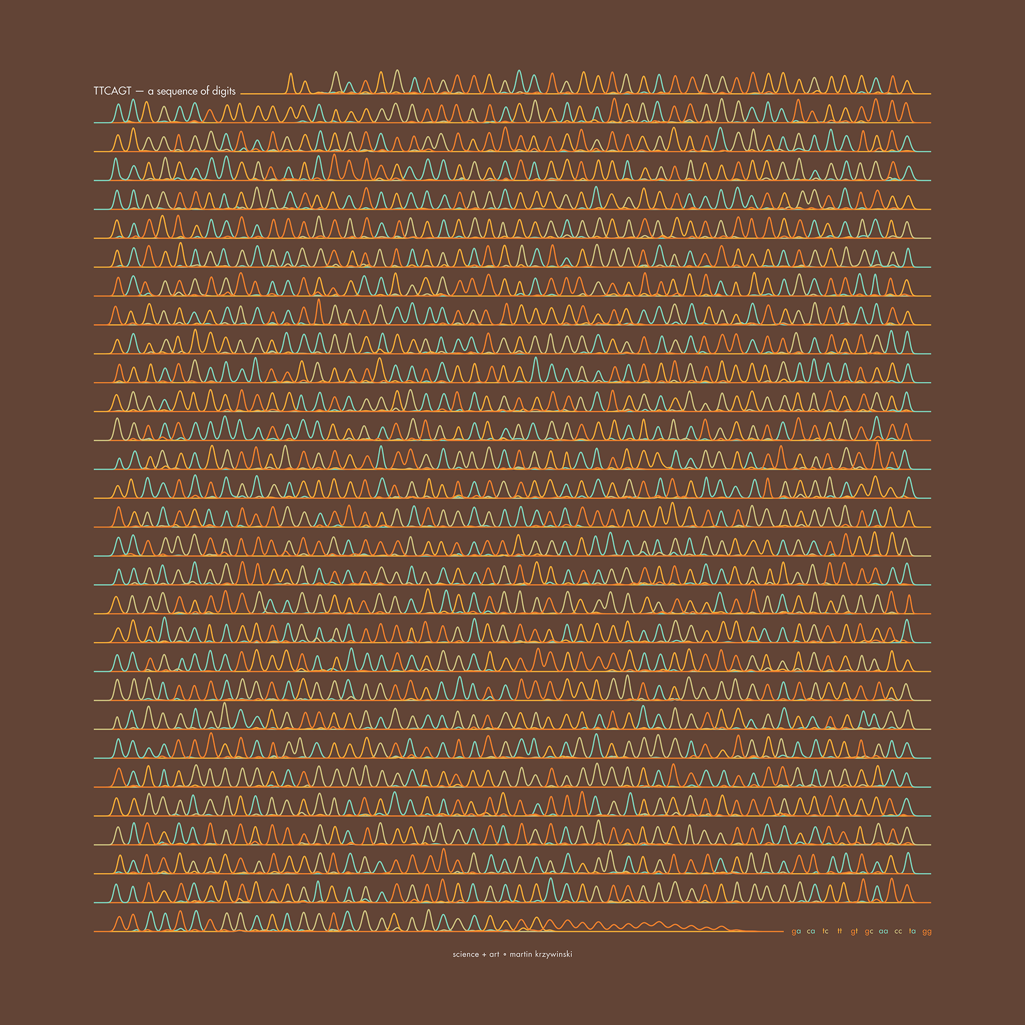
TTCAGT: a sequence of digits
Celebrate π Day (March 14th) and sequence digits like its 1999. Let's call some peaks.
Crafting 10 Years of Statistics Explanations: Points of Significance
I don’t have good luck in the match points. —Rafael Nadal, Spanish tennis player
Points of Significance is an ongoing series of short articles about statistics in Nature Methods that started in 2013. Its aim is to provide clear explanations of essential concepts in statistics for a nonspecialist audience. The articles favor heuristic explanations and make extensive use of simulated examples and graphical explanations, while maintaining mathematical rigor.
Topics range from basic, but often misunderstood, such as uncertainty and P-values, to relatively advanced, but often neglected, such as the error-in-variables problem and the curse of dimensionality. More recent articles have focused on timely topics such as modeling of epidemics, machine learning, and neural networks.
In this article, we discuss the evolution of topics and details behind some of the story arcs, our approach to crafting statistical explanations and narratives, and our use of figures and numerical simulations as props for building understanding.
Altman, N. & Krzywinski, M. (2025) Crafting 10 Years of Statistics Explanations: Points of Significance. Annual Review of Statistics and Its Application 12:69–87.
Propensity score matching
I don’t have good luck in the match points. —Rafael Nadal, Spanish tennis player
In many experimental designs, we need to keep in mind the possibility of confounding variables, which may give rise to bias in the estimate of the treatment effect.
If the control and experimental groups aren't matched (or, roughly, similar enough), this bias can arise.
Sometimes this can be dealt with by randomizing, which on average can balance this effect out. When randomization is not possible, propensity score matching is an excellent strategy to match control and experimental groups.
Kurz, C.F., Krzywinski, M. & Altman, N. (2024) Points of significance: Propensity score matching. Nat. Methods 21:1770–1772.
Understanding p-values and significance
P-values combined with estimates of effect size are used to assess the importance of experimental results. However, their interpretation can be invalidated by selection bias when testing multiple hypotheses, fitting multiple models or even informally selecting results that seem interesting after observing the data.
We offer an introduction to principled uses of p-values (targeted at the non-specialist) and identify questionable practices to be avoided.
Altman, N. & Krzywinski, M. (2024) Understanding p-values and significance. Laboratory Animals 58:443–446.