visualization + design
Hilbert Curve Art, Hilbertonians and Monkeys
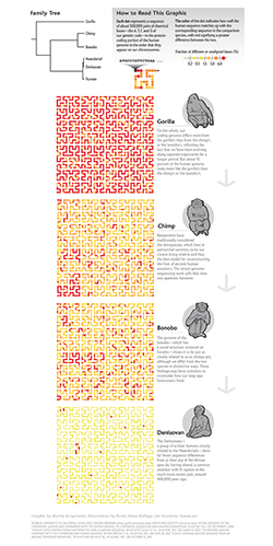
I collaborated with Scientific American to create a data graphic for the September 2014 issue. The graphic compared the genomes of the Denisovan, bonobo, chimp and gorilla, showing how our own genomes are almost identical to the Denisovan and closer to that of the bonobo and chimp than the gorilla.
Here you'll find Hilbert curve art, a introduction to Hilbertonians, the creatures that live on the curve, an explanation of the Scientific American graphic and downloadable SVG/EPS Hilbert curve files.
monkey genomes
This page accompanies my blog post at Scientific American, which itself accompanies the figure in the magazine.
In the blog post I argue that the genome is not a blueprint—a common metaphor that doesn't leave room for appreciating the complexity of the genome—and talk about the process of creating the figure.
the graphic
brief
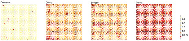
The graphic shows the differences between the genome sequence of human and each of Denisovan, chimp, bonobo and gorilla. Differences are measured by the fraction of bases in the gene regions of human sequence that do not align to the other genome.
The approximately 1 Gb of sequence of gene regions (most introns are included) is divided into 2,047 bins which are mapped onto the Hilbert curve as circles.
The color of the circle, which represents about 500 kb of sequence, encodes the fraction of unaligned bases.
The original color scheme submitted for production was derived from the yellow-orange-red Brewer palette.
measuring differences
There's more than one way to do it.
The approach taken by the graphic is one of the simplest—this is why it was chosen. It's easy to understand and easy to explain. On the other hand, the answer depends on the state of the sequence resources for each species (especially bonobo, whose sequence assembly is in version 1) and completely overlooks the functional implications of these differences.
The real goal of identifying differences, a relatively superficial problem, is to find the subset of differences that make a difference, which is a deep problem.
For example, if someone told you that Vancouver, Canada and Sydney, Australia were 85% similar, you would likely assume that (a) this metric isn't that useful to you unless it aligns to your priorities in how city similarities should be judged, (b) other metrics would give different answers, and (c) some parts of Sydney are nothing like Vancouver while others might be identical. This goes the same for genomes, except that cities are easier to figure out since we built them ourselves.
The differences will be scattered throughout the genome and will take many forms: single base changes, small insertions or deletions, inversions, copy number changes, and so on. In parts critical to basic cell function we expect no differences (e.g. insulin gene exons) while in genes that are rapidly evolving we expect to see some differences.
A comparison of protein coding genes reveals approximately 500 genes showing accelerated evolution on each of the gorilla, human and chimpanzee lineages, and evidence for parallel acceleration, particularly of genes involved in hearing.
— Insights into hominid evolution from the gorilla genome sequence by Scally et al.
Parts of the genome that don't impact function are going to accumulate differences at a background rate of mutation.
uncertainty in life sciences
Any single-number statistic that compares two genomes is necessarily going to be a gross approximation. Such numerical measures should be taken as a starting point and at best as some kind of average that hides all of the texture in the data.
Statements like "the 1% difference" are incomplete because they do not incorporate an uncertainty. If you see four separate reports claiming a 1%, 2%, 5% and 7% difference, this does not necessarily mean that we cannot agree. It means that the error in our measurement is large. You might venture a guess that the answer is somewhere in the range 1–7% (at the very least).
While confidence intervals and error bars are a sine qua non in physical sciences, assessing uncertainty in life sciences is a lot more difficult. To assess the extent of biological variation, which will add to the uncertainty in our result, we need to collecting data from independent biological samples. Often this is too expensive or not practical.
To provide a sober and practical guide to statistics for the busy biologist, Naomi Altman and myself write the Points of Significance column in Nature Methods. These kinds of resources are needed as long as errors persist in the translation between statistical analysis and conclusions (e.g. `5 sigma` and P values).
We don't yet have a full handle on individual levels of genomic variation, especially for non-human primates for which we have a single and incomplete genome. Even for humans, although we have resources like dbSNP, which catalogue individual variation, it is common to use the canonical human reference sequence for analysis. This reference sequence is only a single instance of a human genome (in fact, parts of it are derived from different individuals).
As a result, many of the reported values (and certainly almost all that make it to popular media) are without any confidence limits and thus are likely to be interpreted as fact rather than as an estimate. This causes all sorts of problems—two compatible estimates can easily (but wrongly) be interpreted as incompatible facts.
As an example, look at the phylogenetic trees in the figure below. Without incorporating uncertainty, the top tree presents a fixed and deceptive state of what we know about the uncertainty in what we know.
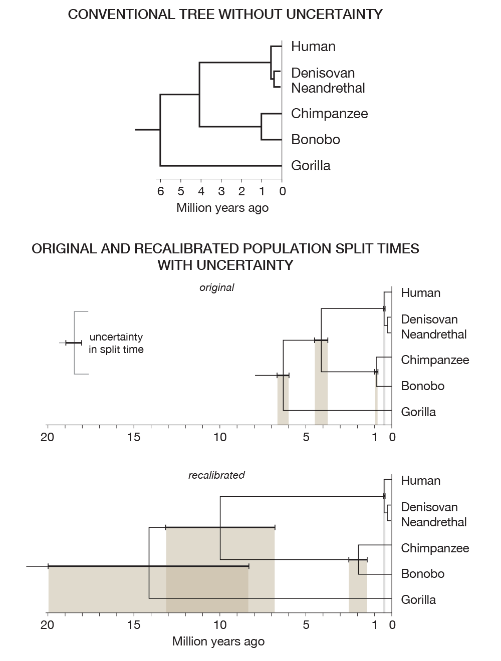
Recent work has shed some light on the uncertainty in determining population split times. The two trees in the figure above are generated from the data in the table below, from 2012 Generation times in wild chimpanzees and gorillas suggest earlier divergence times in great ape and human evolution Proc Natl Acad Sci U S A 109 (39) 15716-15721.
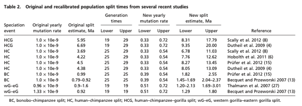
Notice that the human/chimp/gorilla split time uncertainty overlaps the human/chimp split.
The addition of uncertainty is the inevitable consequence of making multiple measurements and upgraded analytical models. It is a blessing not a curse.
when we measure, we estimate
That our genome is "similar" to that of the chimp, bonobo and gorilla is not in dispute. How to classify and quantify the differences is an active field of research, a process that often looks like a dispute.
We have been sequencing quickly and cheaply for less than 10 years. It's amazing how much we've been able to understand in such a short period of time. Genome sequencing (or some kind of genotyping) is now routinely done in the treatment of cancer. It is not long before a medical diagnosis will include an assessment of the full genome sequence.
As we sequence more and reflect more, we expect to change our minds. In fact, this is why we do science: so that our minds are changed.
Scientists engage the public in the process of scientific inquiry, testing and observation by way of reports in popular science media and newspapers. Understanding these reports requires that one holds as a core value to process of science and its outcomes. Groups with different agendas and a fundamentally different epistemology hijaack observations such as "In 30% of the genome, gorilla is closer to human or chimpanzee than the latter are to each other." (from the gorilla sequence paper) in an attempt to argue that our evolutionary models are sinfully wrong. They don't understand the implications of the uncertainty in our measurements (e.g. phylogenetic tree figure above) and have world outlooks that are impervious to the impact of observation.
It is certain that these genomes hold more surprises for us, but not in the way these groups claim.
Is our science incomplete? Absolutely. How do we address this? We do more science.
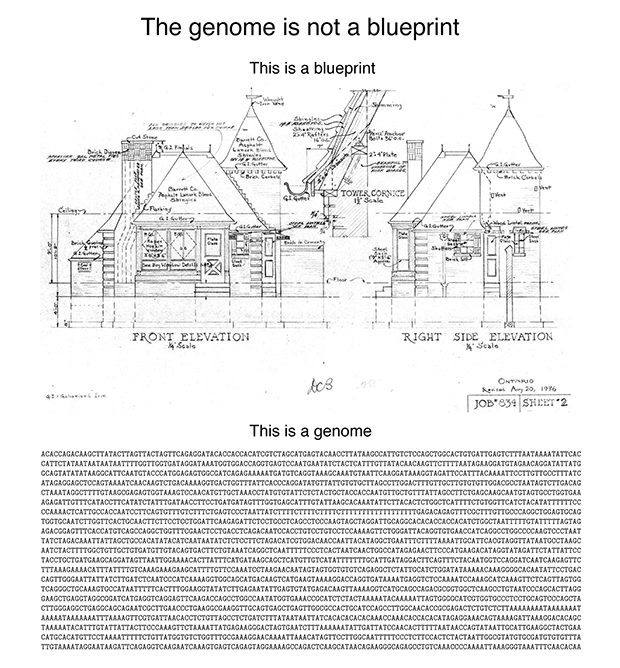
genome is not a blueprint
The genome is not blueprint. It's also absolutely not a recipe, which is promulgated by people who agree that it is not a blueprint. I explain my view of this here and why I think these analogies have disasterous effects on the public understanding of how their genomes (i.e. their bodies) work.
Sometimes metaphors are wonderful and they help expand our mind.
I, a universe of atoms, an atom in the universe.
—Richard Feynman
Other times they are like jailors, keeping us from having productive thoughts.
Genomics: the big blueprint
—nature.com
You might argue that "blueprint" is one of the closest words in meaning, so its use is justified. The trouble is that its actually very far in meaning.
Consider the following figure.
A blueprint shows you "what". A genome doesn’t encode "what". It doesn’t even encode “how”. Nor does it encode "from what". It encodes "with what", which is several degrees removed from "what". I promise that this will make sense shortly.
The reason why the blueprint analogy is pernicious is that it makes it sound like once the genome sequence is known, the rest easily follows. The reality is that these days the genome sequence is easily determined and the rest follows with great effort (or never) (see The $1,000 genome, the $100,000 analysis? by Elaine Mardis).
I'm going to try to motivate you that the analogy is false by an example. Suppose that you wanted to build a house but instead of getting blueprints from the architect, you received this strange drawing.
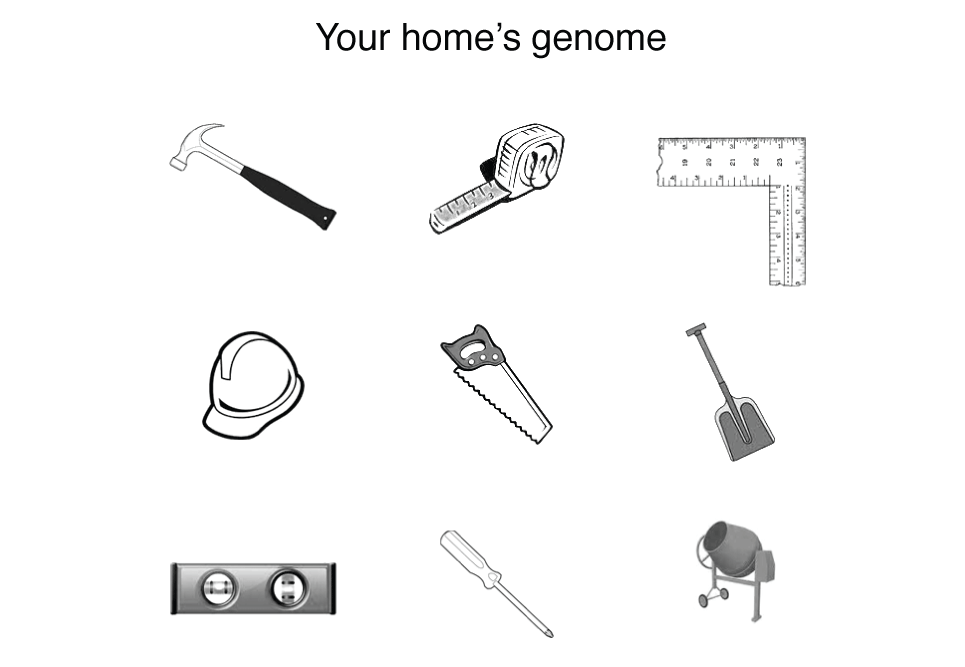
You’d be right to be confused—welcome to genome science. This house’s genome looks a lot like a set of tools and bears no resemblance to the house itself. The genome tells you nothing about (a) what the function of each tool is, (b) the effect of the tools form to its function (e.g. what are the many ways in which a hammer can diverge from its original shape before it ceases to be useful), (c) what the tools act on (this is why above I said "with what" rather than "from what"), (d) how the tools act together, and importantly (e) what the tools are used to build.
This is more of a way a genome works. It encodes the protein enzymes that make biochemical reactions possible at room temperature. In the house example, the tools encoded by the genome (e.g. saw, hammer) can be thought of automatically doing their job when they’re in the presence of the correct material (wood, nail). This is in analogy to enzymes, which mediate reactions when in physical proximity of chemical substrates.
Neither wood nor nails—both essential materials for construction—appear anywhere in your home's genome. This directly translates into a biochemical example. We use sugar as a source of energy but the genome hints nothing at this—it only encodes the enzymes that act on sugar. Things are made more complex by the fact that the function of an enzyme is essentially impossible to predict without additional information, such as knowledge of functions of enzymes with similar characteristics.
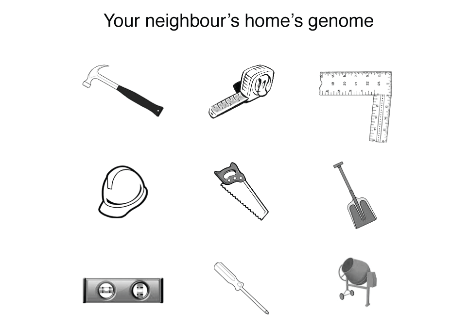
You can probably imagine that the effect of changes in the home's genome is extraordinary difficult to predict. The figure below extends our example to that of your neighbour, which was recently observed to have collapsed. I’ll leave you to work out the mystery yourself.
So next time someone says that the genome is a blueprint, or that it is the "code of life", point out that it is merely the "code of tools" for life, which is the emerging property of a set of chemicals confined within a physical space.
hilbert curve in genomics
The use of the Hilbert curve in genomics is not new. It appeared on the cover of Science in 2009 in connection to the 3-dimensional packing of the genome. It is an order 5 curve and just a flip of the curve I use in the Scientific American graphic. Here the corners of the curve have been smoothed out to give it a more organic and gooey feel.
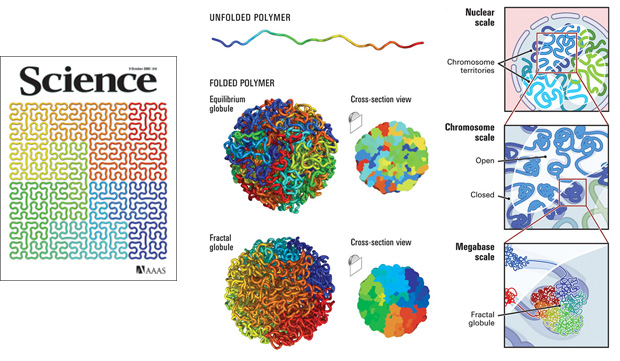
At least one tool exists (HilbertVis) that allows you to wrap genomic data onto the curve.
2009 Visualization of genomic data with the Hilbert curve Bioinformatics 25 (10) 1231-1235.
I've used the Hilbert curve before to show the organization of genes in the genome. This figure shows the chromosome at a much higher resolution than would be possible if an ordinary line was used.

Because the Hilbert curve stretches the line into a square, it increases our ability to see details in data at higher resolution. In the figure below you can see distinct clumpiness in the organization of genes on the chromsome that is not representative of a purely random sampling.

data sources
Except for the Denisovan, the net alignments (e.g. human vs chimp net) from UCSC Genome browser were used for the analysis.
Gaps were intersected with human gene regions. For each gene, the region between the start of the first coding region and end of the last coding region was used.
human (Homo sapiens sapiens)
The RefSeq gene annotation from the UCSC Genome table browser was used. The union of all 51,010 RefSeq gene records was used.
The gene region was taken as the extent of the gene's coding sequence (CDS), not just the exons within it.
For example, for the BRCA2 gene, the RefSeq entry is
                        tx                cds
BRCA2 NM_000059 chr13 + 32889616-32973809 32890597-32972907

                        exons exonstart            exonend
                        27    32889616,32890558... 32889804,32890664...
This record's contribution was the region 32890597-32972907, shown in bold above.
The total size of the union of tx regions is 1.28 Gb (20,722 coverage elements), of cds regions as defined above is 0.99 Gb (24,931 coverage elements) and of exons is 74.5 Mb (225,404 coverage elements).
Assembly version: Feb 2009 (CRCh37/hg19)
Denisovan
30x sequence was aligned to the human genome at Max Planck (data portal).
chimp (Pan troglodytes)
Assembly version: Feb 2011 (panTro4)
bonobo (Pan paniscus)
Assembly version: May 2012 (panPan1).
At the moment this genome is available only on the test version of the browser.
Assembly version: Feb 2009 (CRCh37/hg19)
gorilla (Gorilla gorilla gorilla)
Assembly version: May 2011 (gorGor3.1/gorGor3)
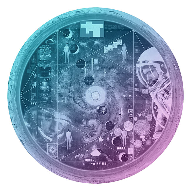
Nasa to send our human genome discs to the Moon
We'd like to say a ‘cosmic hello’: mathematics, culture, palaeontology, art and science, and ... human genomes.

Comparing classifier performance with baselines
All animals are equal, but some animals are more equal than others. —George Orwell
This month, we will illustrate the importance of establishing a baseline performance level.
Baselines are typically generated independently for each dataset using very simple models. Their role is to set the minimum level of acceptable performance and help with comparing relative improvements in performance of other models.
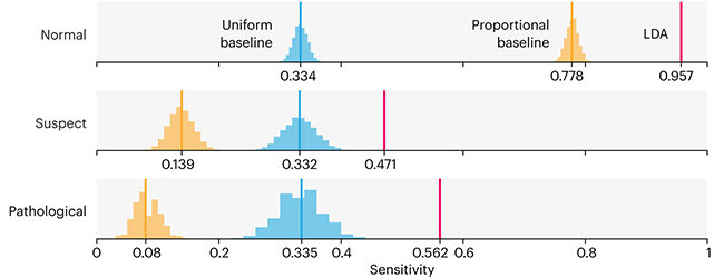
Unfortunately, baselines are often overlooked and, in the presence of a class imbalance5, must be established with care.
Megahed, F.M, Chen, Y-J., Jones-Farmer, A., Rigdon, S.E., Krzywinski, M. & Altman, N. (2024) Points of significance: Comparing classifier performance with baselines. Nat. Methods 20.
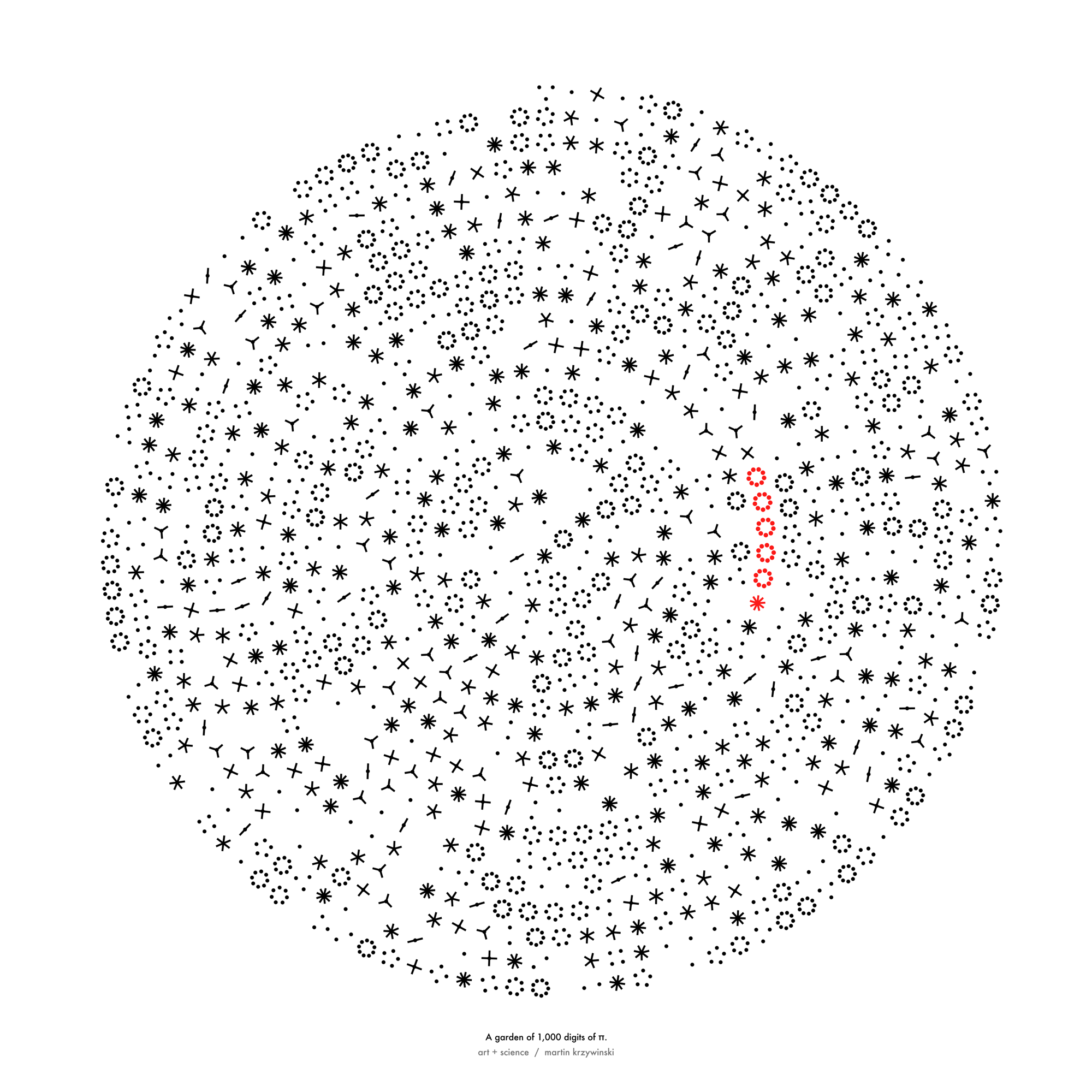
Happy 2024 π Day—
sunflowers ho!
Celebrate π Day (March 14th) and dig into the digit garden. Let's grow something.
How Analyzing Cosmic Nothing Might Explain Everything
Huge empty areas of the universe called voids could help solve the greatest mysteries in the cosmos.
My graphic accompanying How Analyzing Cosmic Nothing Might Explain Everything in the January 2024 issue of Scientific American depicts the entire Universe in a two-page spread — full of nothing.
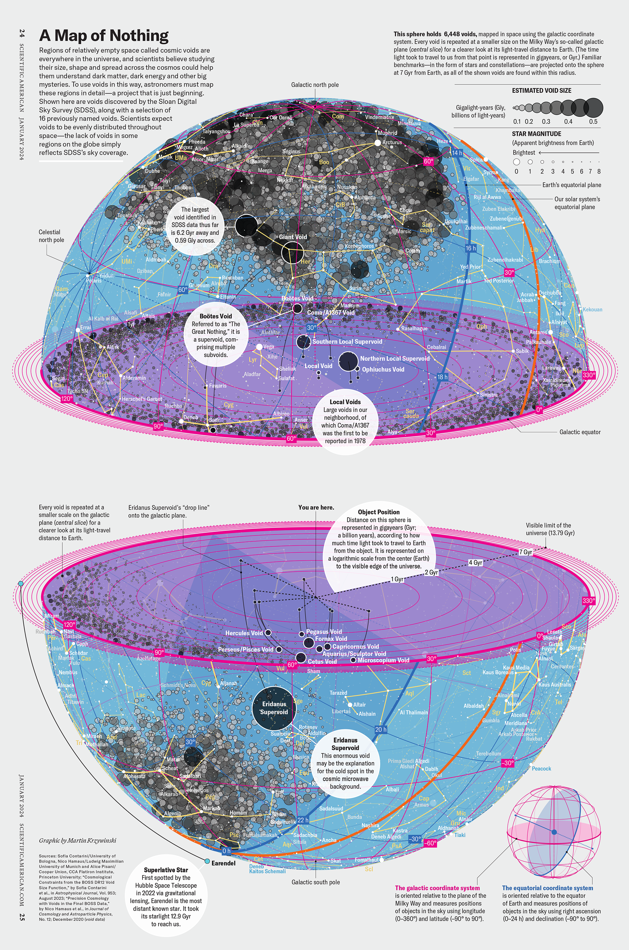
The graphic uses the latest data from SDSS 12 and is an update to my Superclusters and Voids poster.
Michael Lemonick (editor) explains on the graphic:
“Regions of relatively empty space called cosmic voids are everywhere in the universe, and scientists believe studying their size, shape and spread across the cosmos could help them understand dark matter, dark energy and other big mysteries.
To use voids in this way, astronomers must map these regions in detail—a project that is just beginning.
Shown here are voids discovered by the Sloan Digital Sky Survey (SDSS), along with a selection of 16 previously named voids. Scientists expect voids to be evenly distributed throughout space—the lack of voids in some regions on the globe simply reflects SDSS’s sky coverage.”
voids
Sofia Contarini, Alice Pisani, Nico Hamaus, Federico Marulli Lauro Moscardini & Marco Baldi (2023) Cosmological Constraints from the BOSS DR12 Void Size Function Astrophysical Journal 953:46.
Nico Hamaus, Alice Pisani, Jin-Ah Choi, Guilhem Lavaux, Benjamin D. Wandelt & Jochen Weller (2020) Journal of Cosmology and Astroparticle Physics 2020:023.
Sloan Digital Sky Survey Data Release 12
Alan MacRobert (Sky & Telescope), Paulina Rowicka/Martin Krzywinski (revisions & Microscopium)
Hoffleit & Warren Jr. (1991) The Bright Star Catalog, 5th Revised Edition (Preliminary Version).
H0 = 67.4 km/(Mpc·s), Ωm = 0.315, Ωv = 0.685. Planck collaboration Planck 2018 results. VI. Cosmological parameters (2018).
constellation figures
stars
cosmology
Error in predictor variables
It is the mark of an educated mind to rest satisfied with the degree of precision that the nature of the subject admits and not to seek exactness where only an approximation is possible. —Aristotle
In regression, the predictors are (typically) assumed to have known values that are measured without error.
Practically, however, predictors are often measured with error. This has a profound (but predictable) effect on the estimates of relationships among variables – the so-called “error in variables” problem.
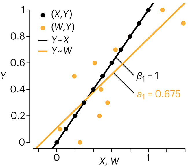
Error in measuring the predictors is often ignored. In this column, we discuss when ignoring this error is harmless and when it can lead to large bias that can leads us to miss important effects.
Altman, N. & Krzywinski, M. (2024) Points of significance: Error in predictor variables. Nat. Methods 20.
Background reading
Altman, N. & Krzywinski, M. (2015) Points of significance: Simple linear regression. Nat. Methods 12:999–1000.
Lever, J., Krzywinski, M. & Altman, N. (2016) Points of significance: Logistic regression. Nat. Methods 13:541–542 (2016).
Das, K., Krzywinski, M. & Altman, N. (2019) Points of significance: Quantile regression. Nat. Methods 16:451–452.
Convolutional neural networks
Nature uses only the longest threads to weave her patterns, so that each small piece of her fabric reveals the organization of the entire tapestry. – Richard Feynman
Following up on our Neural network primer column, this month we explore a different kind of network architecture: a convolutional network.
The convolutional network replaces the hidden layer of a fully connected network (FCN) with one or more filters (a kind of neuron that looks at the input within a narrow window).
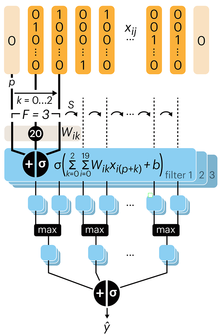
Even through convolutional networks have far fewer neurons that an FCN, they can perform substantially better for certain kinds of problems, such as sequence motif detection.
Derry, A., Krzywinski, M & Altman, N. (2023) Points of significance: Convolutional neural networks. Nature Methods 20:1269–1270.
Background reading
Derry, A., Krzywinski, M. & Altman, N. (2023) Points of significance: Neural network primer. Nature Methods 20:165–167.
Lever, J., Krzywinski, M. & Altman, N. (2016) Points of significance: Logistic regression. Nature Methods 13:541–542.
Neural network primer
Nature is often hidden, sometimes overcome, seldom extinguished. —Francis Bacon
In the first of a series of columns about neural networks, we introduce them with an intuitive approach that draws from our discussion about logistic regression.
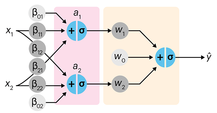
Simple neural networks are just a chain of linear regressions. And, although neural network models can get very complicated, their essence can be understood in terms of relatively basic principles.
We show how neural network components (neurons) can be arranged in the network and discuss the ideas of hidden layers. Using a simple data set we show how even a 3-neuron neural network can already model relatively complicated data patterns.
Derry, A., Krzywinski, M & Altman, N. (2023) Points of significance: Neural network primer. Nature Methods 20:165–167.
Background reading
Lever, J., Krzywinski, M. & Altman, N. (2016) Points of significance: Logistic regression. Nature Methods 13:541–542.
Cell Genomics cover
Our cover on the 11 January 2023 Cell Genomics issue depicts the process of determining the parent-of-origin using differential methylation of alleles at imprinted regions (iDMRs) is imagined as a circuit.
Designed in collaboration with with Carlos Urzua.
Akbari, V. et al. Parent-of-origin detection and chromosome-scale haplotyping using long-read DNA methylation sequencing and Strand-seq (2023) Cell Genomics 3(1).
Browse my gallery of cover designs.
Science Advances cover
My cover design on the 6 January 2023 Science Advances issue depicts DNA sequencing read translation in high-dimensional space. The image showss 672 bases of sequencing barcodes generated by three different single-cell RNA sequencing platforms were encoded as oriented triangles on the faces of three 7-dimensional cubes.
More details about the design.

Kijima, Y. et al. A universal sequencing read interpreter (2023) Science Advances 9.
Browse my gallery of cover designs.
Regression modeling of time-to-event data with censoring
If you sit on the sofa for your entire life, you’re running a higher risk of getting heart disease and cancer. —Alex Honnold, American rock climber
In a follow-up to our Survival analysis — time-to-event data and censoring article, we look at how regression can be used to account for additional risk factors in survival analysis.
We explore accelerated failure time regression (AFTR) and the Cox Proportional Hazards model (Cox PH).
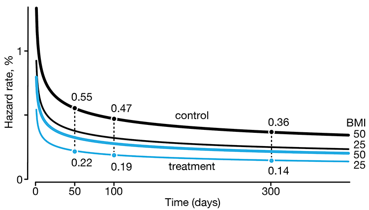
Dey, T., Lipsitz, S.R., Cooper, Z., Trinh, Q., Krzywinski, M & Altman, N. (2022) Points of significance: Regression modeling of time-to-event data with censoring. Nature Methods 19:1513–1515.