
Science Advances Cover
6 January 2023, Issue 9, Volume 1
contents
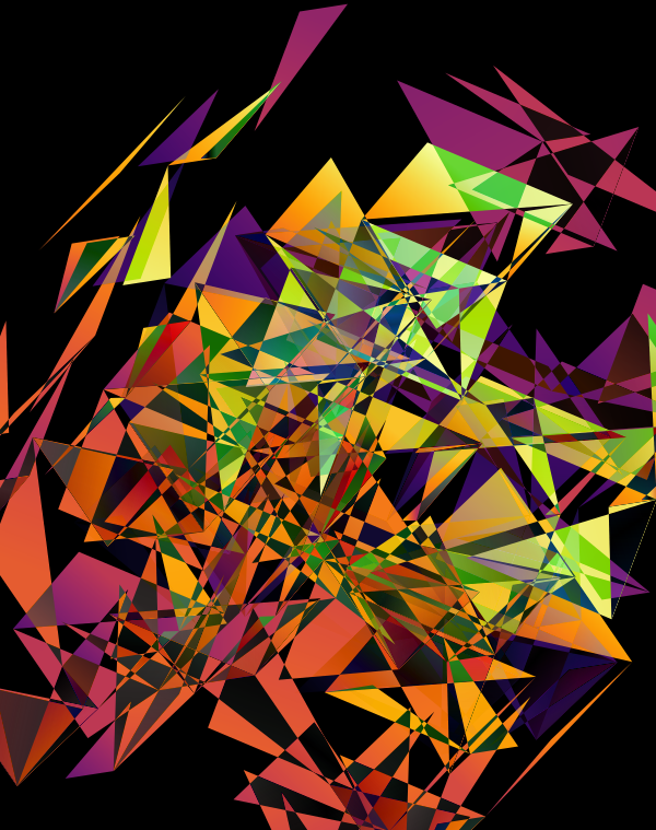
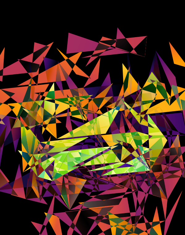
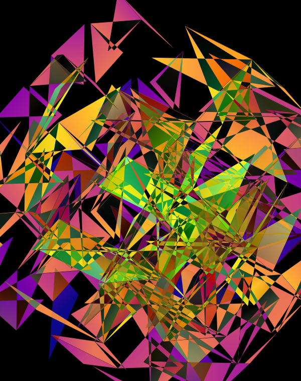
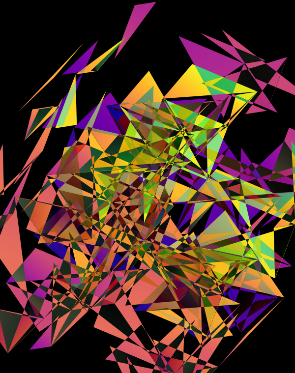
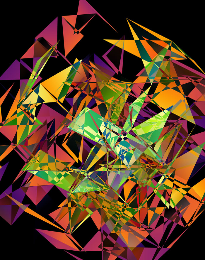
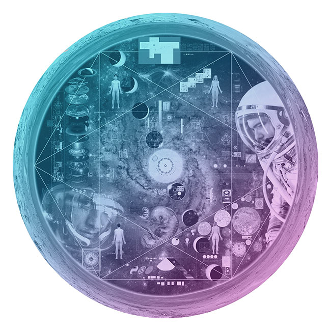
The cover design accompanies the publication of INTERSTELLAR — Kijima, Y. et al. A universal sequencing read interpreter (2023) Science Advances 9. — a kind of universal sequencing read interpreter. Its role is to convert sequencing reads from one sequencing platform to another.
The need for this arises because each platform has a different format for its barcodes that store single cell, spatial and molecular identifiers.
Given that INTERSTELLAR is a kind of “Rosetta Stone” for reads, I thought it would be interesting to try to create something that looked like a puzzle, while encoding barcode sequences from various platforms.
For example, here are some sets of barcodes that all store the same information but vary only by their format.
# 10X, quartz and drop-seq barcodes
ATGAAAGAGCGGGTATCCTTAGTCTTCA TACTACGGTTACGGTGTCTTTT AAAAGGTGTAAATTAACCAC
CCGTGAGAGTTCTGGCCCAGACTTTATT TTACCGTGGCCTCTTTGCTAGG AAAGTGCCACAACTGCGGAA
GCATGATGTCAAGCAGTGCAGGTCCTTG TCTCACTTCACTCCGCTCGCGG AAAATCAGTACGCGGAGTGA
GAGAGGTTCCCAATAGCTCTGCTATGGC ACTTCAATTCTGCCGTATATAT AAATCCATAGAGGGCCACGA
GTGTCCTCAGACAGCATGGTTTATTCGC GCGCAATAGTCTCCAGGGGCGG AAATGGGGTCAGCCAGTTCG
...
Barcode bases are encoded onto the 2-dimensional faces of hypercubes by oriented triangles.
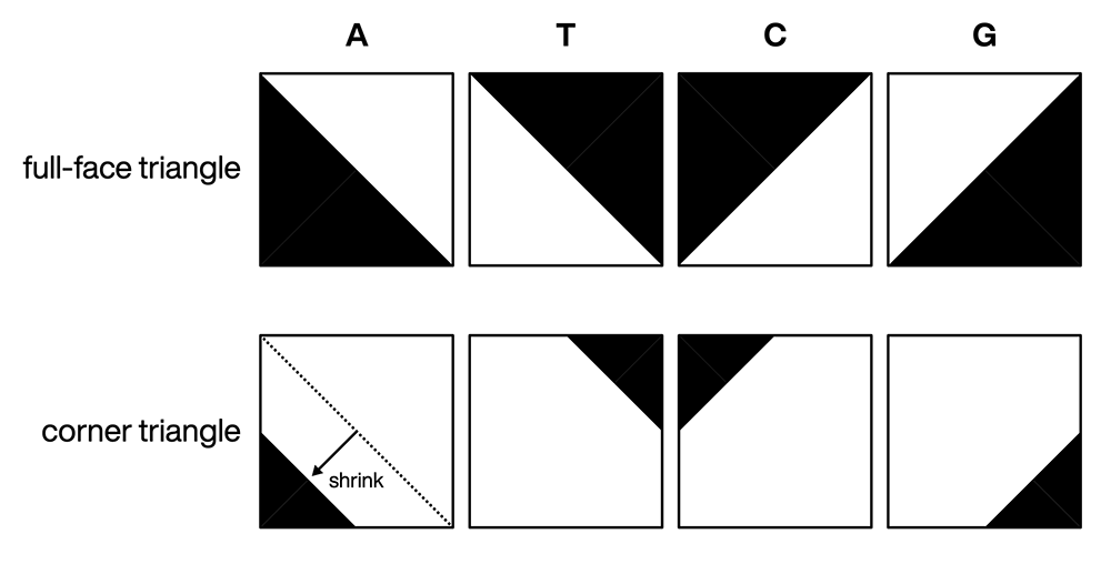
Bases are assigned to faces by traversing the faces in order of the coordinates that correspond to the face's plane.
For example, suppose we want to encode ATGAAA onto a 3-dimensional cube. The cube has 6 faces, which we enumerate as follows
[0] xy x,y,0 A
[1] xy x,y,1 T
[2] xz x,0,z G
[3] xz x,1,z A
[4] yz 0,y,z A
[5] yz 1,y,z A
The first is the face in the `xy` plane at `z=0`, the second in the `xy` plane at `z=1`. We then advance to the next dimension for the second component of the plane coordinate — bringing us to the `xz` plane at `y=0` and `y=1`.
When we go to higher dimensions, the sample process applies. Except now, we have more faces — `2^d` for `d` dimensions. For example, a `d=5` cube has 80 faces to which we can encode 80 bases as follows.
[0]xy000A [1]xy001T [2]xy010G [3]xy011A [4]xy100A [5]xy101A [6]xy110G [7]xy111A [8]x0z00G [9]x0z01C [10]x0z10G [11]x0z11G [12]x1z00G [13]x1z01T [14]x1z10A [15]x1z11T [16]x00u0C [17]x00u1C [18]x01u0T [19]x01u1T [20]x10u0A [21]x10u1G [22]x11u0T [23]x11u1C [24]x000vT [25]x001vT [26]x010vC [27]x011vA [28]x100vC [29]x101vC [30]x110vG [31]x111vT [32]0yz00G [33]0yz01A [34]0yz10G [35]0yz11A [36]1yz00G [37]1yz01T [38]1yz10T [39]1yz11C [40]0y0u0T [41]0y0u1G [42]0y1u0G [43]0y1u1C [44]1y0u0C [45]1y0u1C [46]1y1u0A [47]1y1u1G [48]0y00vA [49]0y01vC [50]0y10vT [51]0y11vT [52]1y00vT [53]1y01vA [54]1y10vT [55]1y11vT [56]00zu0G [57]00zu1C [58]01zu0A [59]01zu1T [60]10zu0G [61]10zu1A [62]11zu0T [63]11zu1G [64]00z0vT [65]00z1vC [66]01z0vA [67]01z1vA [68]10z0vG [69]10z1vC [70]11z0vA [71]11z1vG [72]000uvT [73]001uvG [74]010uvC [75]011uvA [76]100uvG [77]101uvG [78]110uvT [79]111uvC
Here, I've shortened how a face is described. For example xy011A is the face in the `xy` plane at `z=0, u=1, v=1` on which we encode an A.
Given a hypercube whose faces encode a sequence, to decode the sequence we need to know the orientation of unit axes in space. This allows us to figure out the coordinates of each vertex.
Once we have the coordinates, we traverse the faces in the order described above and look at its triangle. If the triangle has a corner at `[0,0]` of the face plane, then the base is an A. If the triangle has a corner at [0,1]`, it's a C. And so on.
For example, a face x0z11 will be a square in the `xz` plane. If we see a tringle corner at `(x,z) = (0,0)`, then we have an A.
You can't easily decode the sequence from a 2-dimensional image of a cube — even if the coordinate axes were shown, some faces would be hidden by others in the image (especially as the number of dimensions is increased).
The code that creates the images is based on the work I did for Max Cooper's Ascent video from his Unspoken Words album.
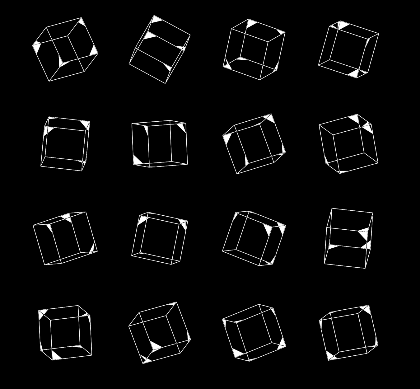
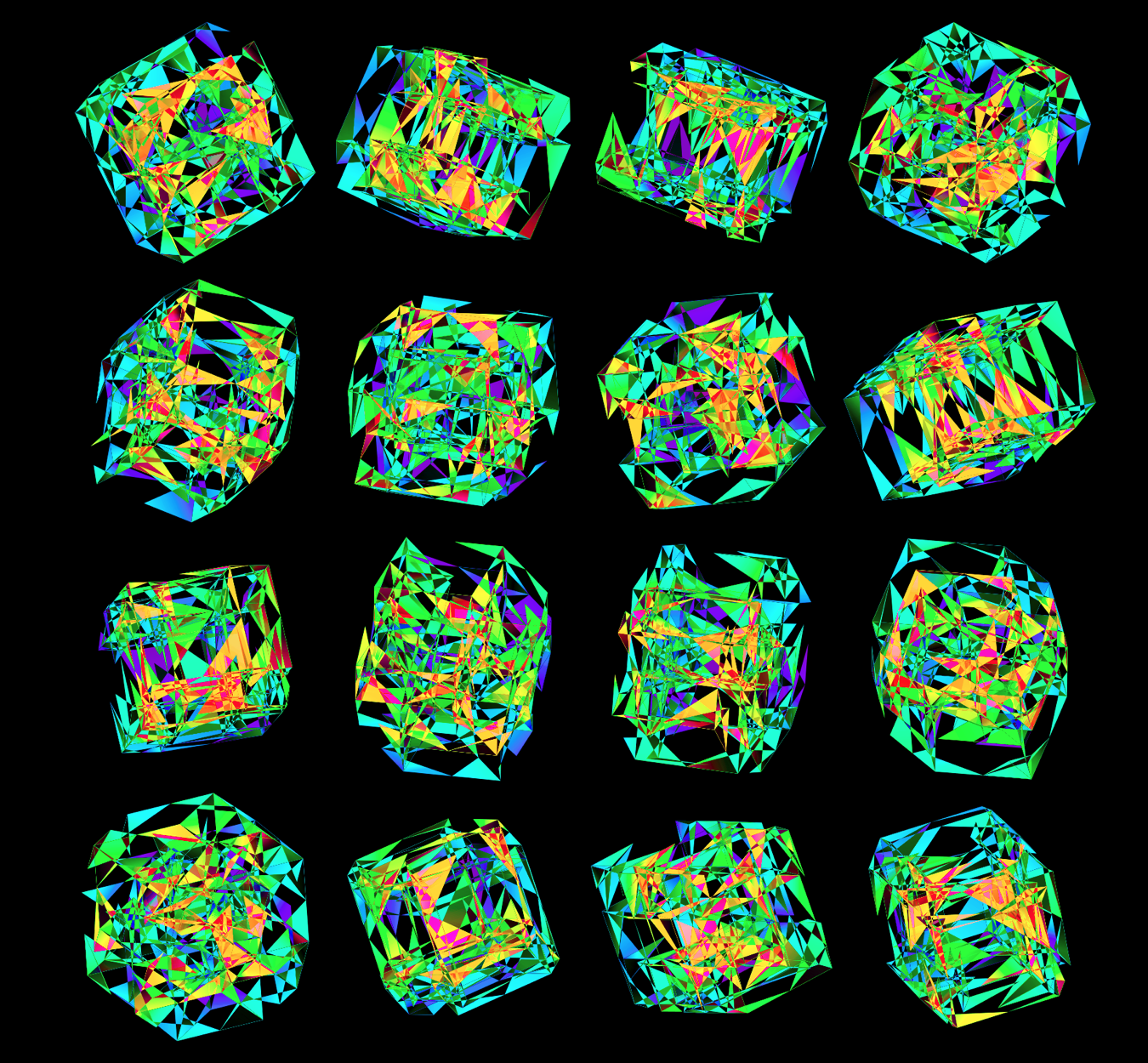
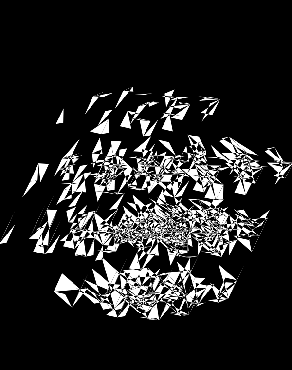
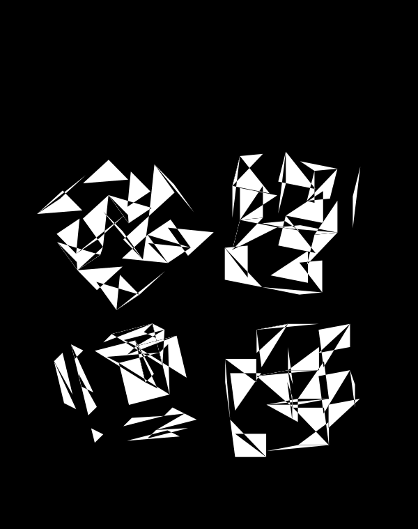
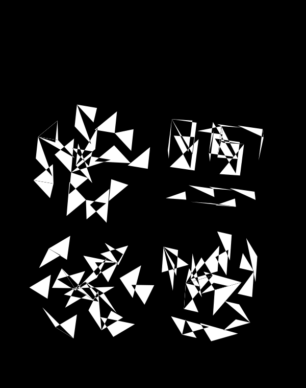
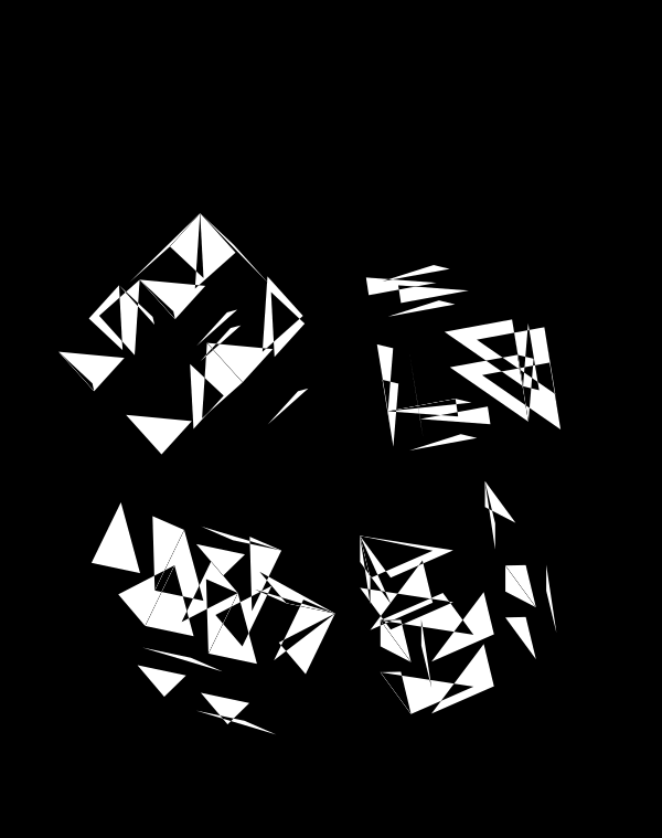
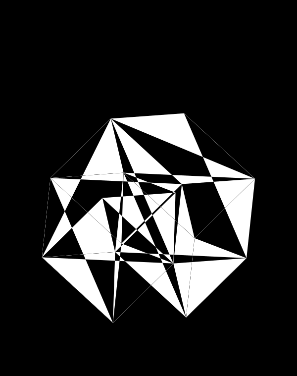
Below, I'll walk through some early prototypes of the design. Each shows an array of 4 × 4 cubes encoding random sequence. Each cube is randomly rotated.
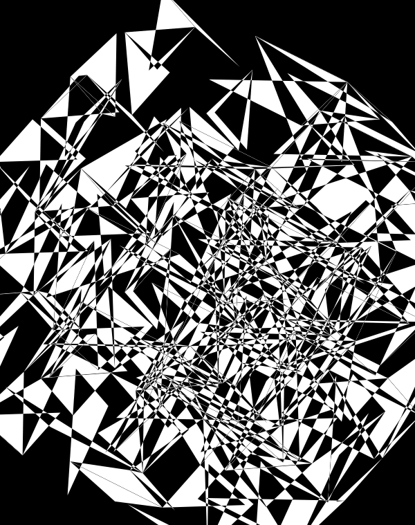
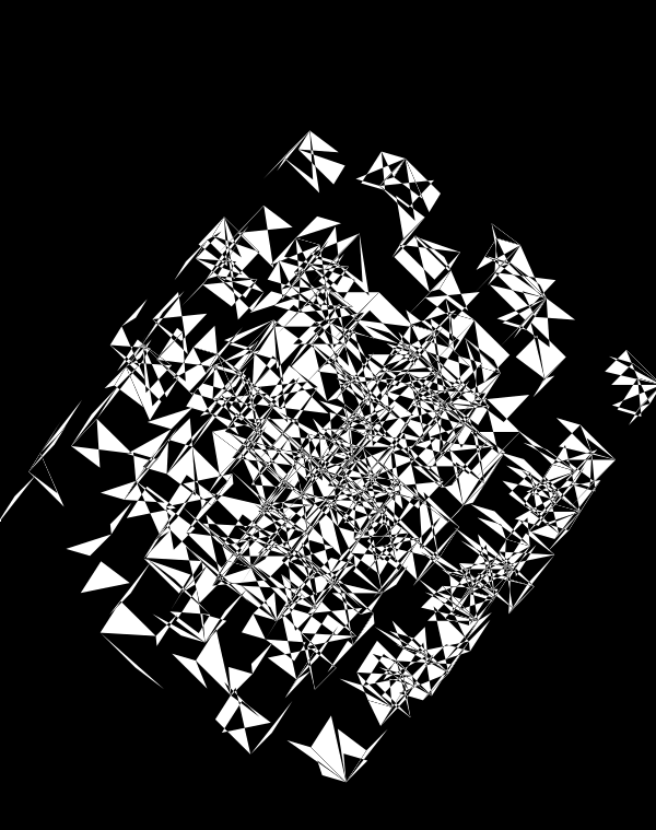
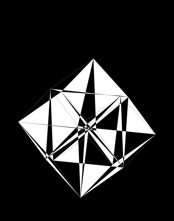
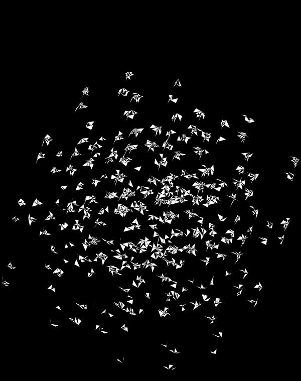
Even with only black and white, if I use a difference blend (e.g. white on white makes black, and vice versa), interesting patterns emerge.
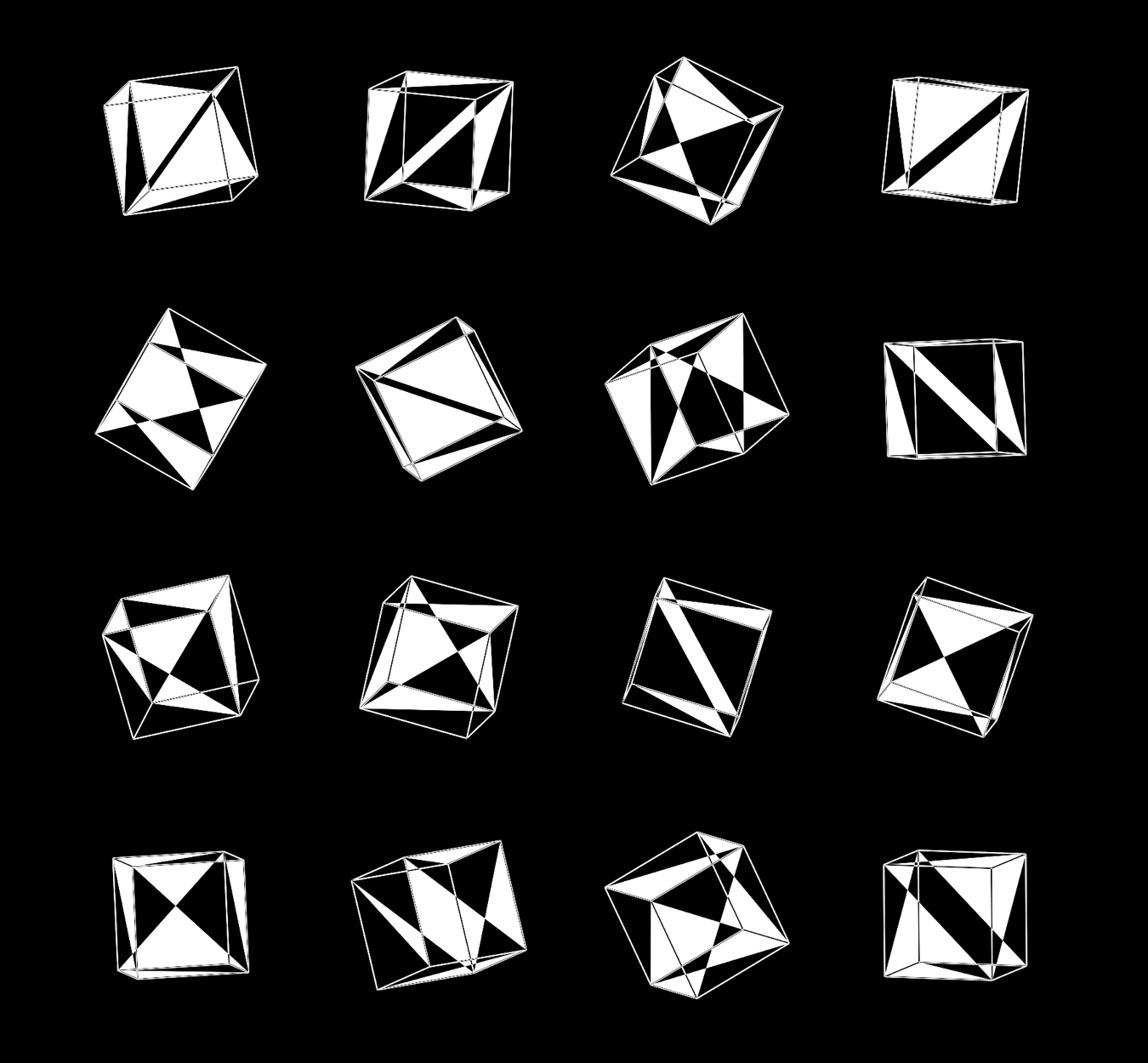
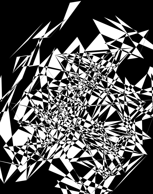
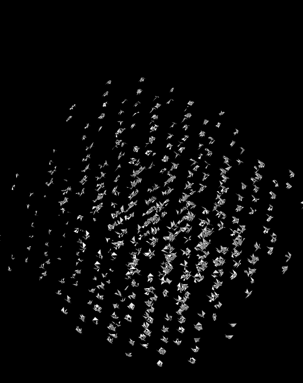
If I start to shrink the triangles towards their corners (here by 50%), the design gains space and the arrangements of triangles becomes even more interesting.
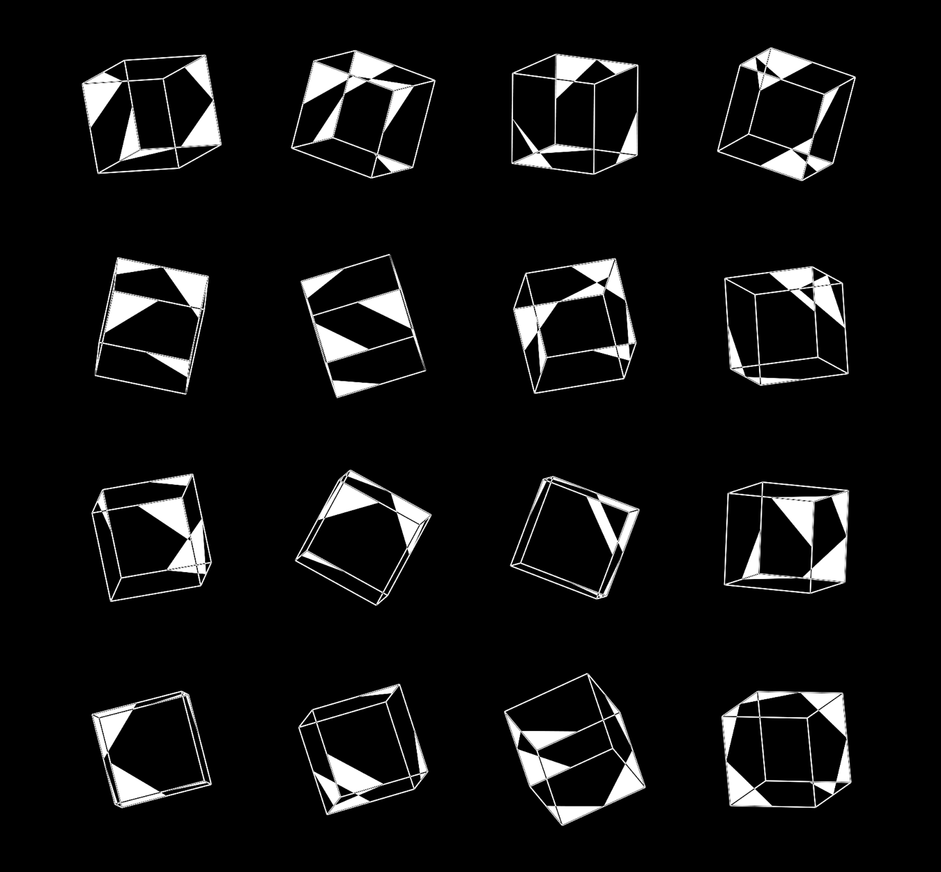
Shrinking the triangles even more (by 75%), we start to see even more room — perfect to accomodate more dimensions.
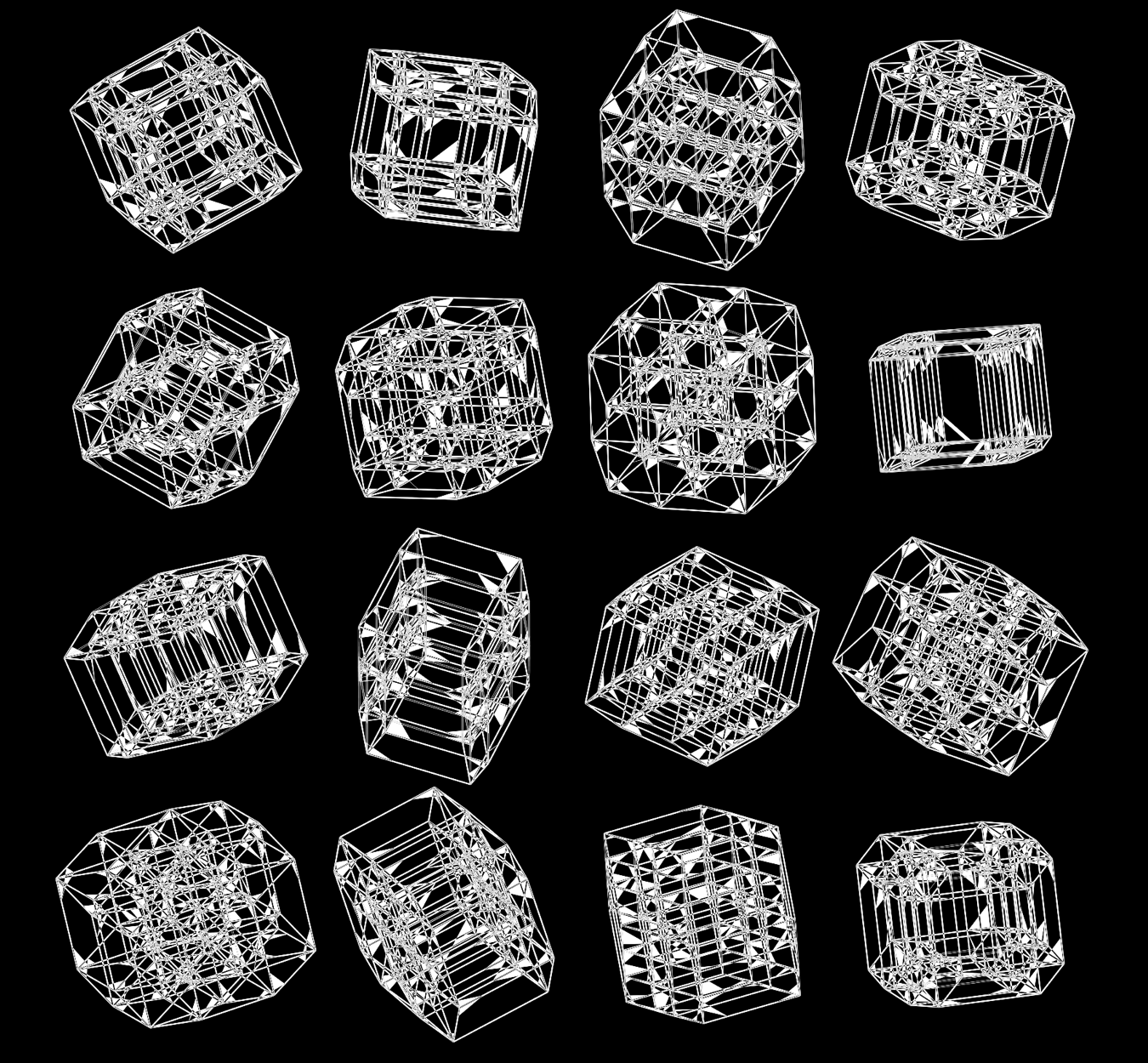
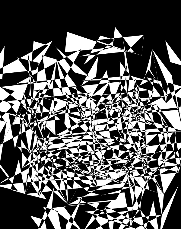
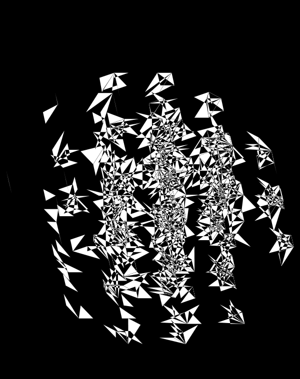
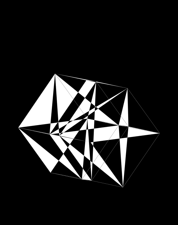
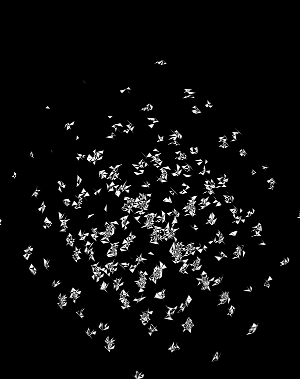
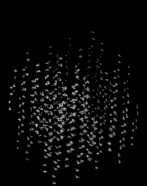
When we go to `d=6` dimensions, our cubes now have 192 faces. In this image, edges are also drawn. You can see how diverse the 2-dimensional projections are. These images are very similar to the scene at 1:44 in the Ascent video, with the only difference being that Ascent uses `d=5` and (at this point in the video) the cube corners have not yet appeared.
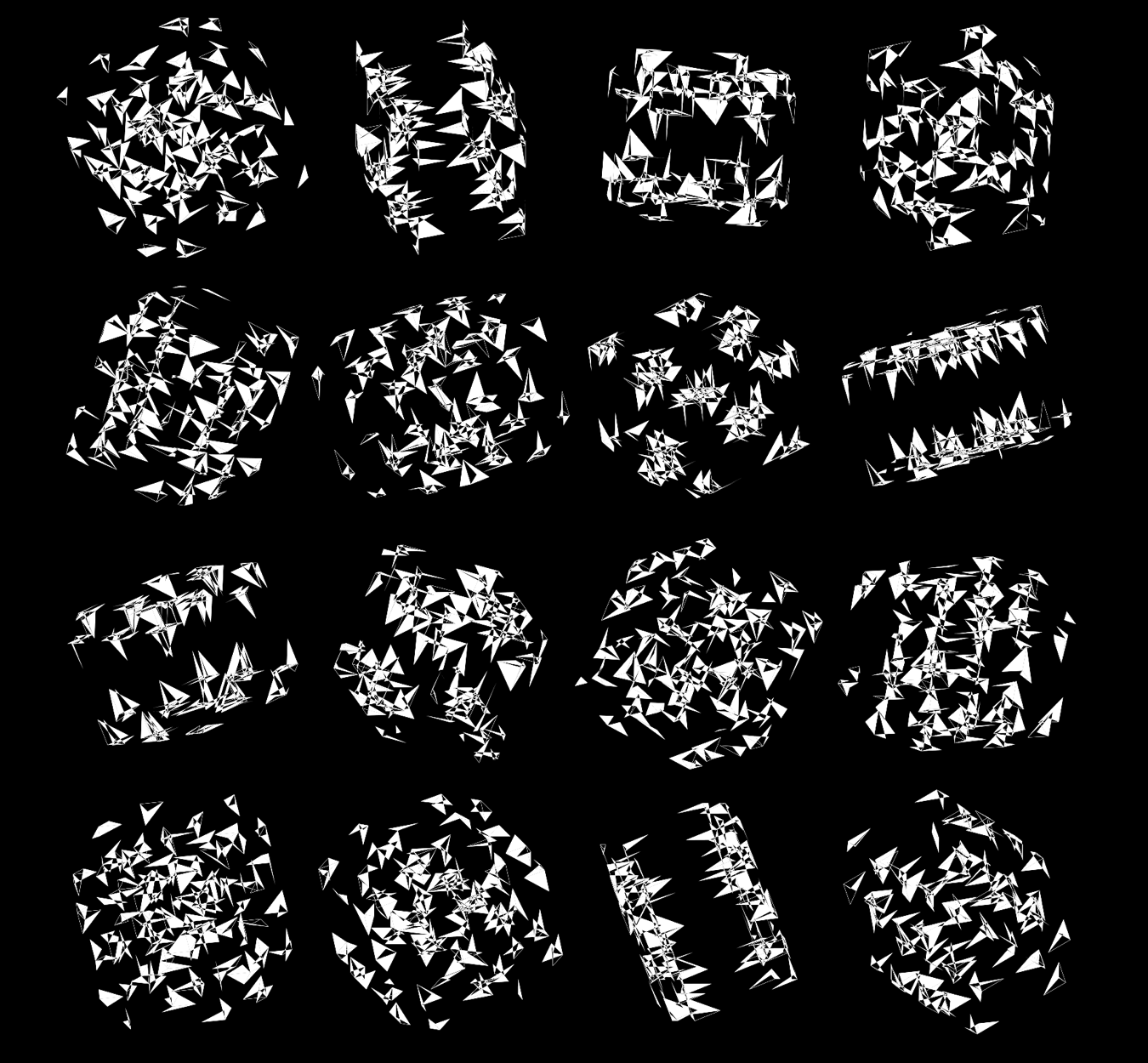
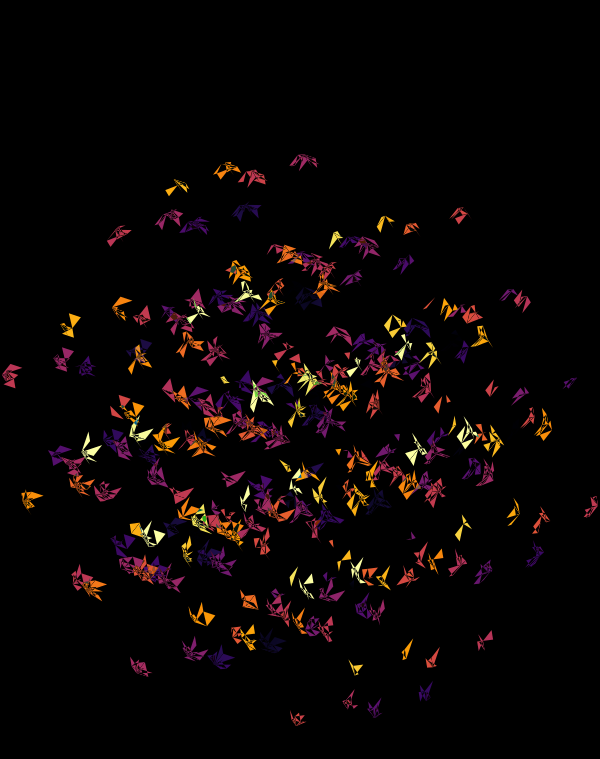
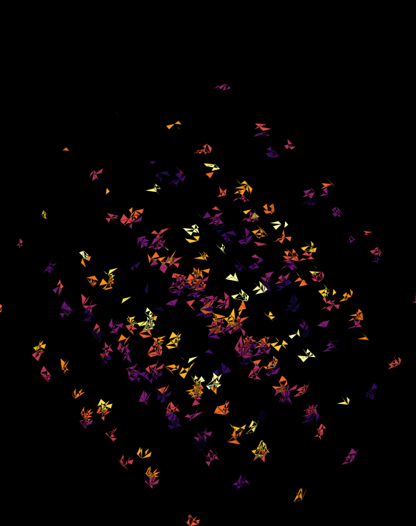
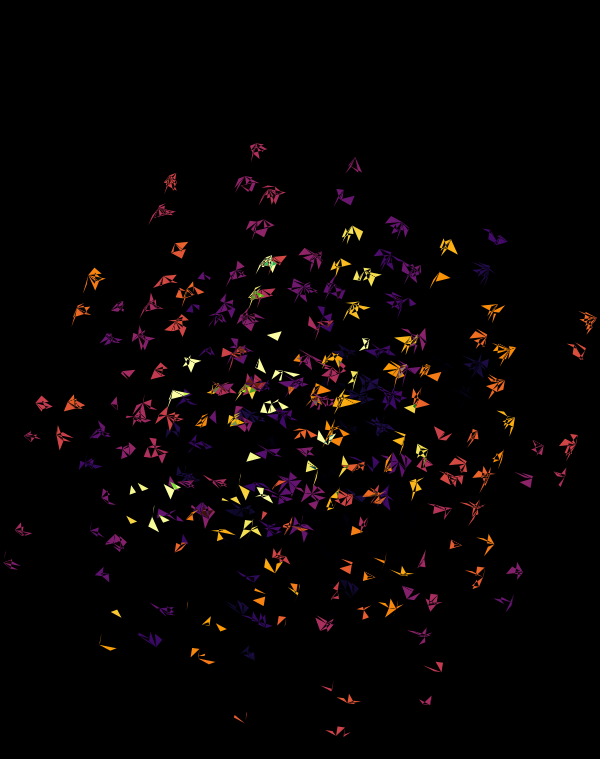
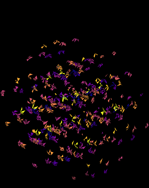
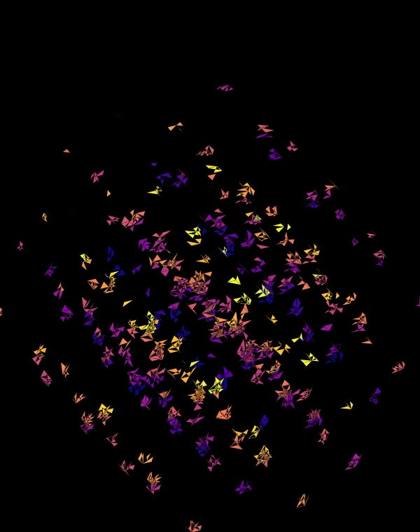
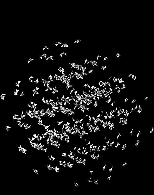
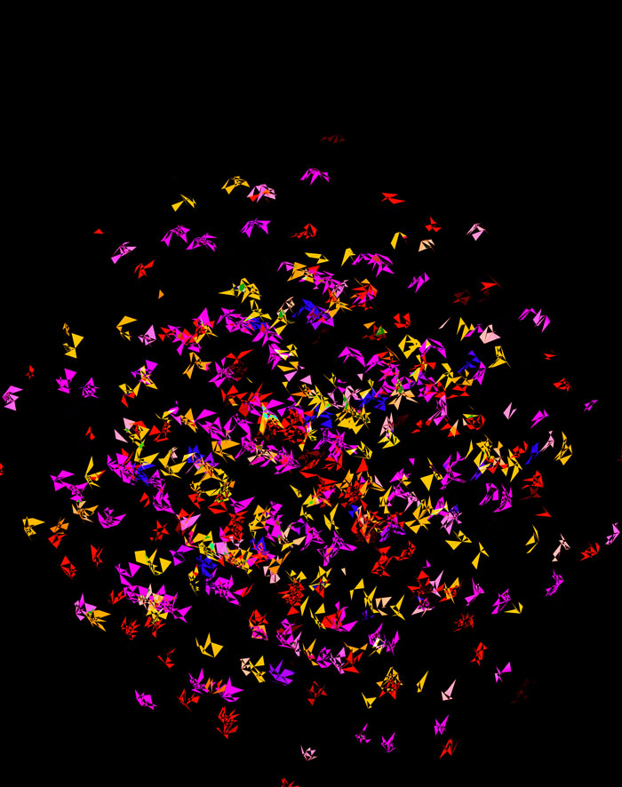
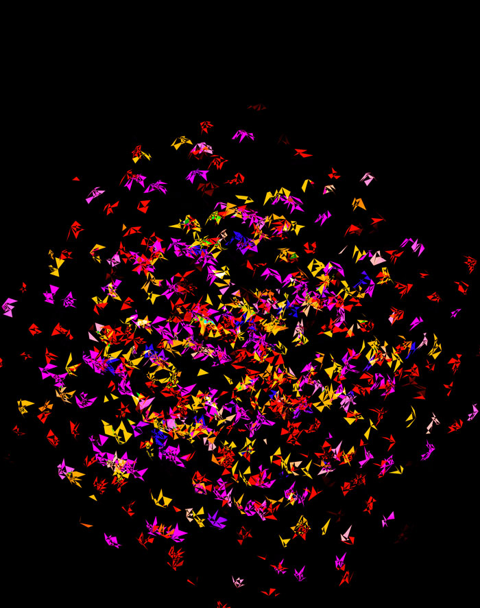
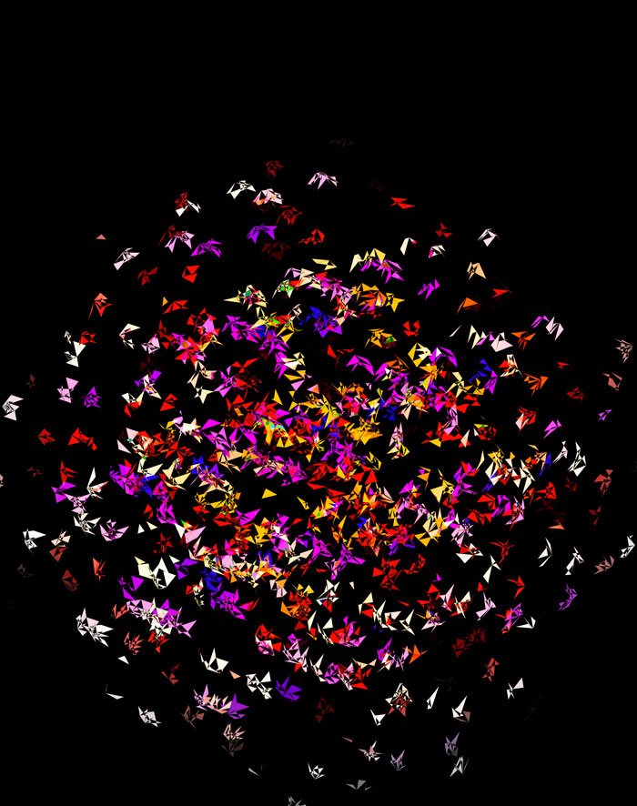
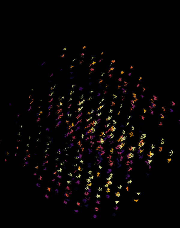
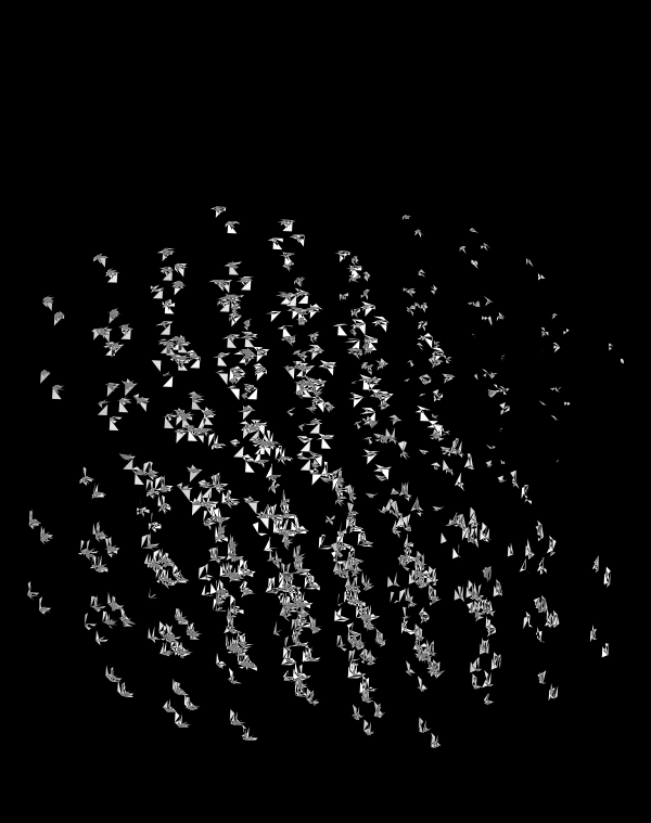
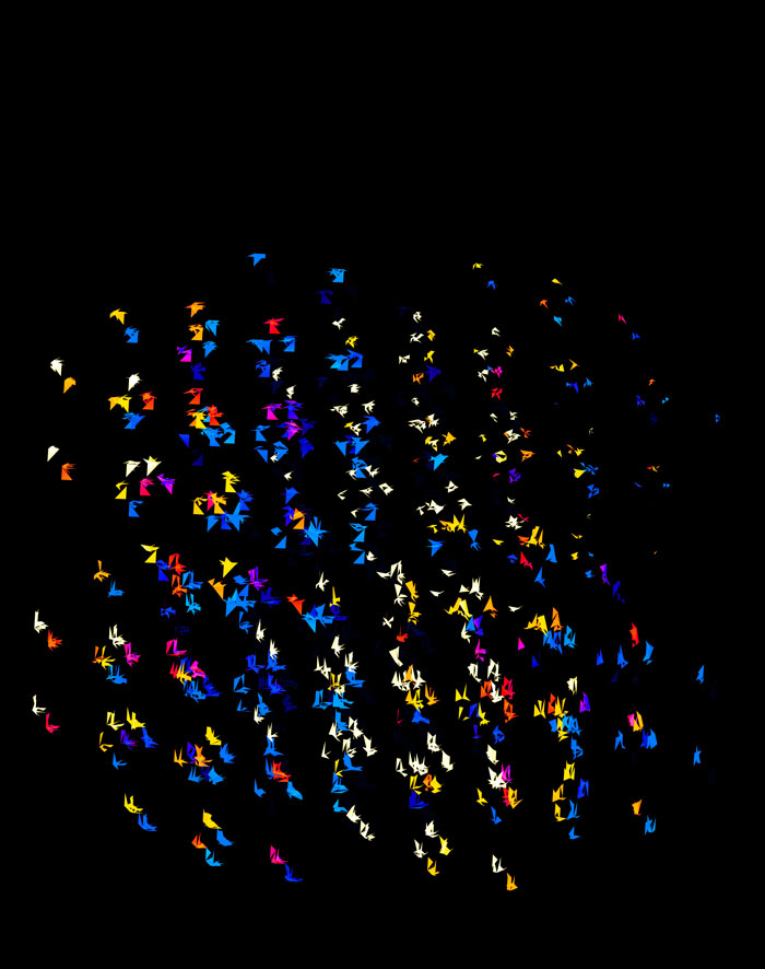
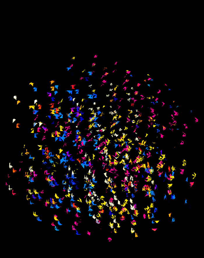
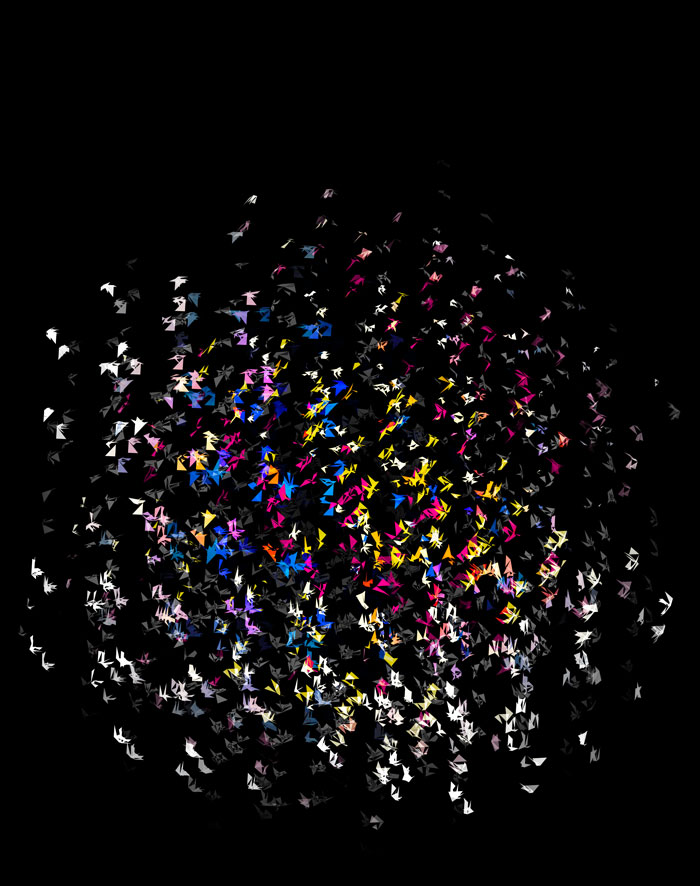
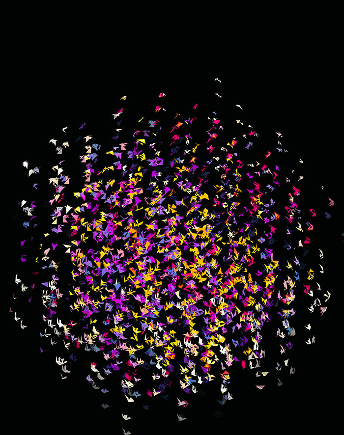
Once we hide the edges, the corners, how by themselves, give a sense of a flock of birds.
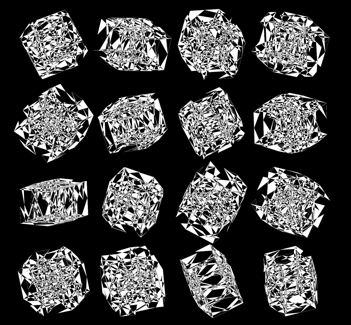
Rich complexity in the patterns arise when we enlarge the triangles ‐ here shrunk by only 50%.
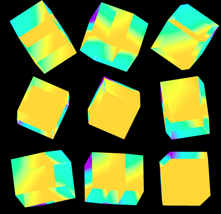
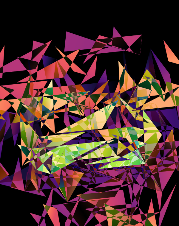
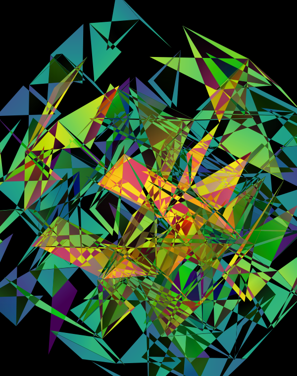
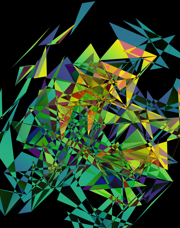
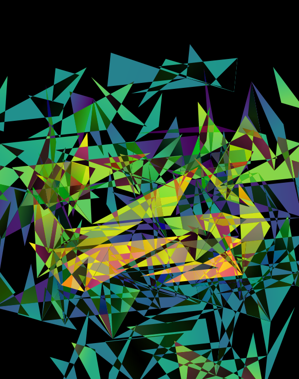
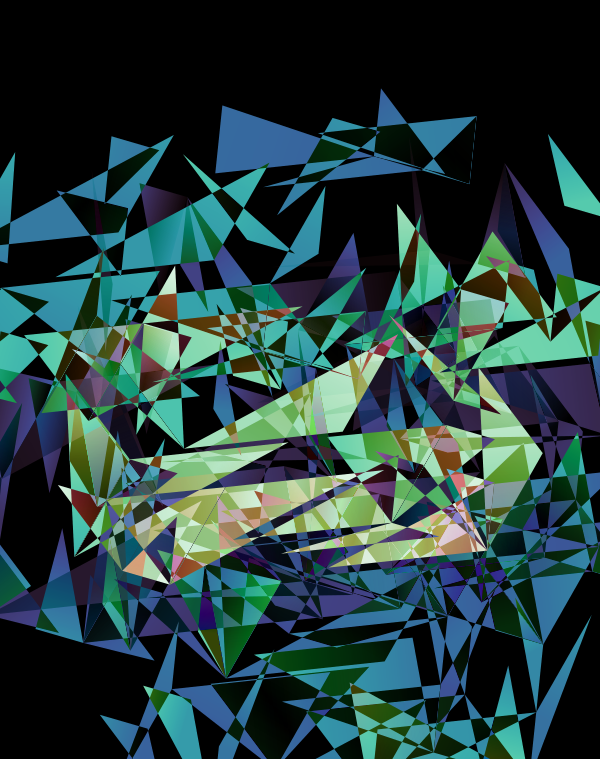
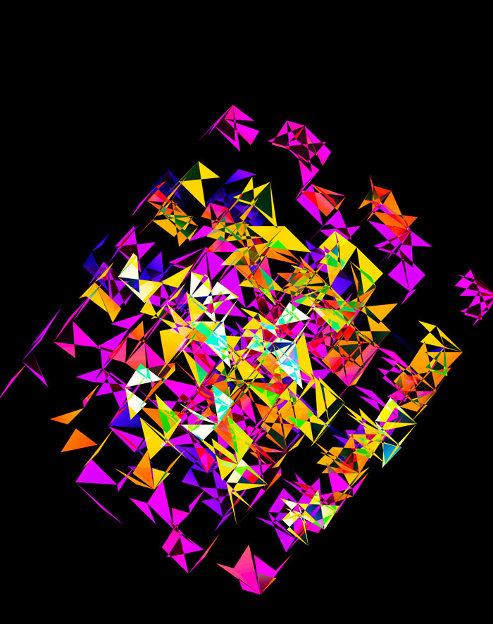
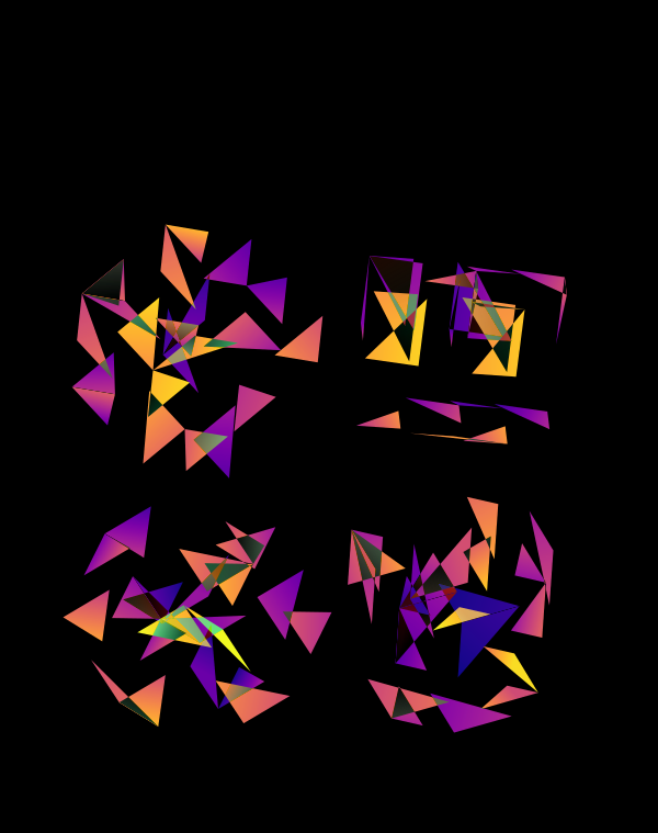
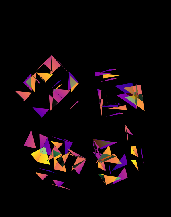
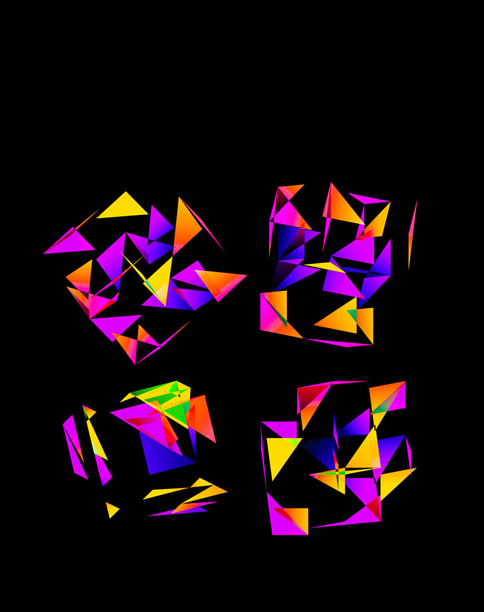
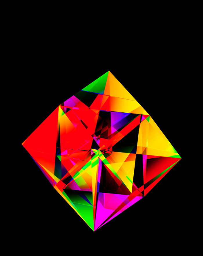
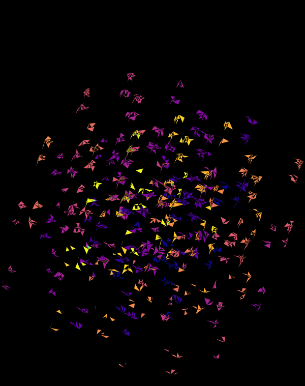
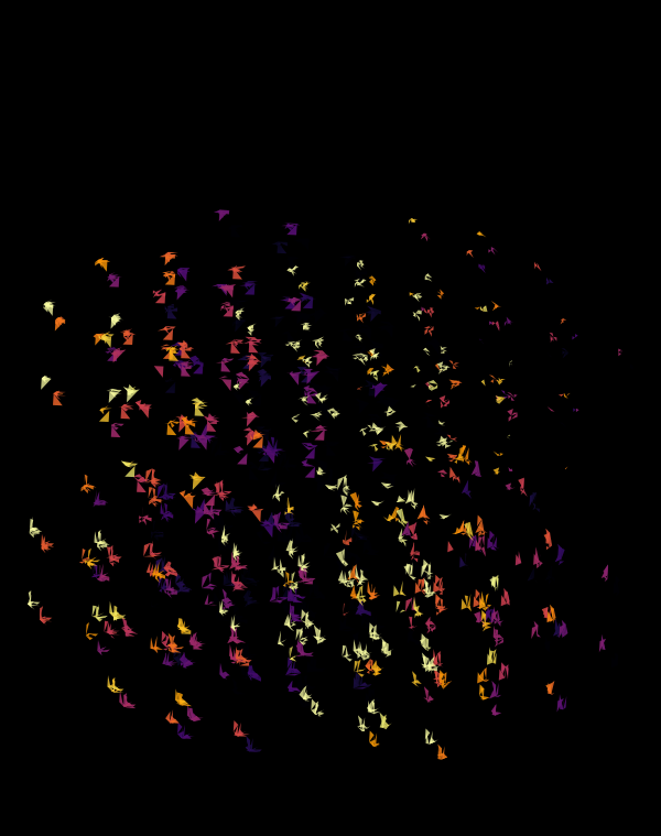
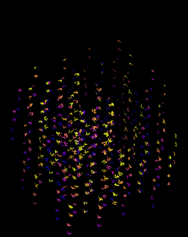
Time for some color. I took the viridis color maps and filled the triangles with a gradient that mapped their z coordinate.
Below are takes that use the viridis color map with half- and full-sized triangles.
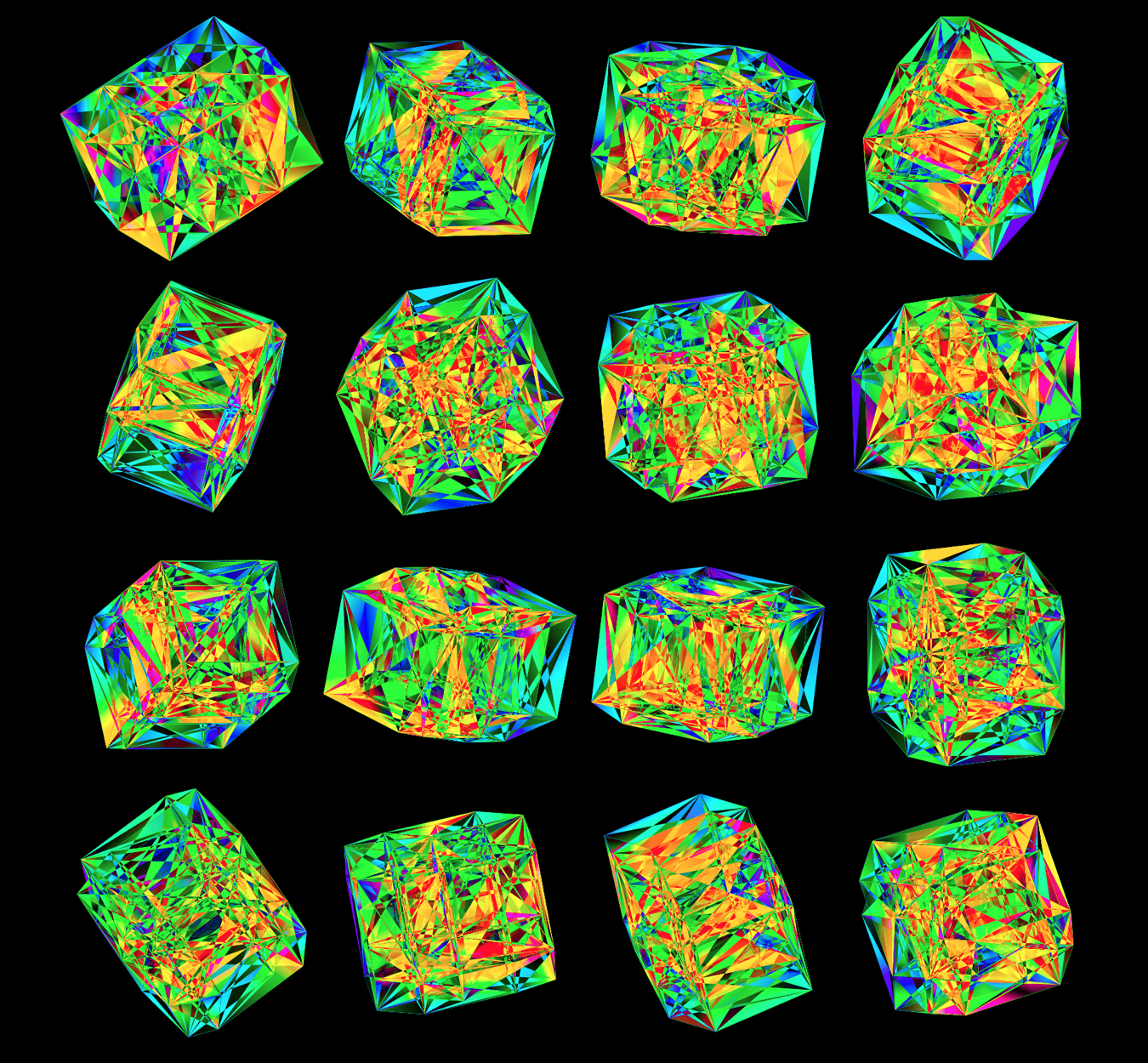
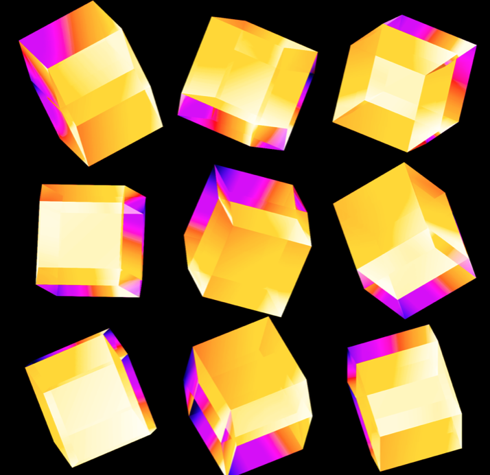
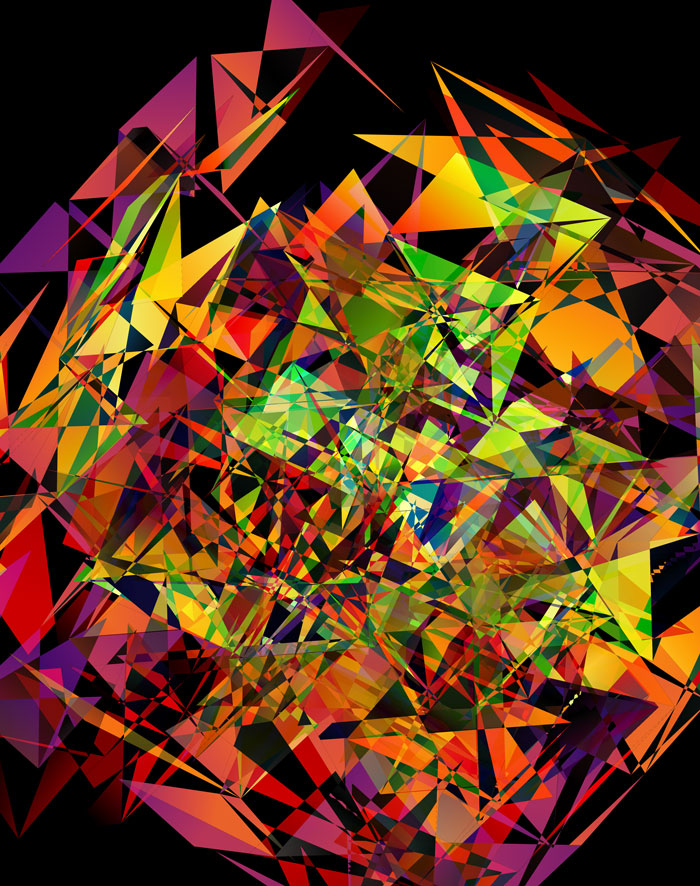
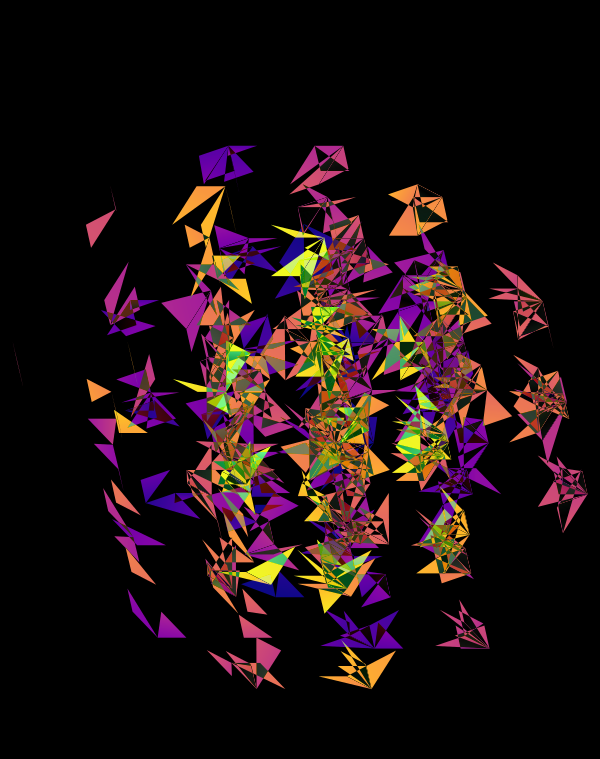
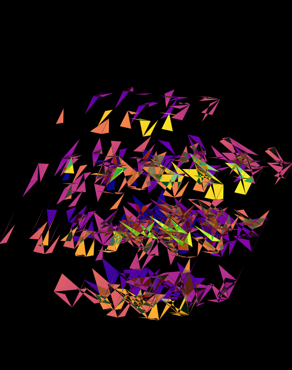
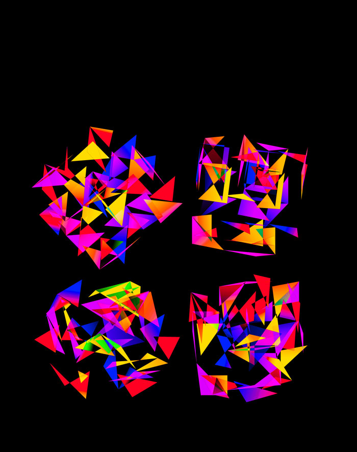
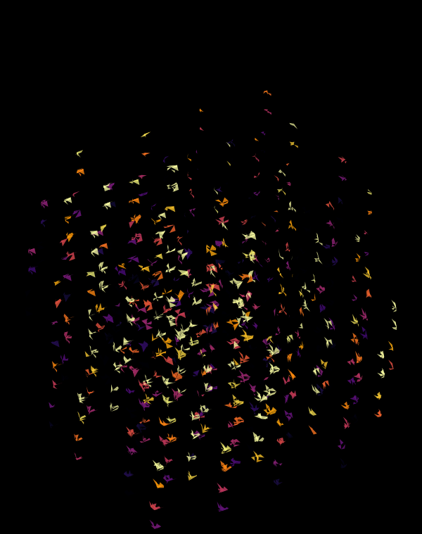
While I found the viridis scheme to be a little too cold, the inferno palette feld just the right amount of warmth.
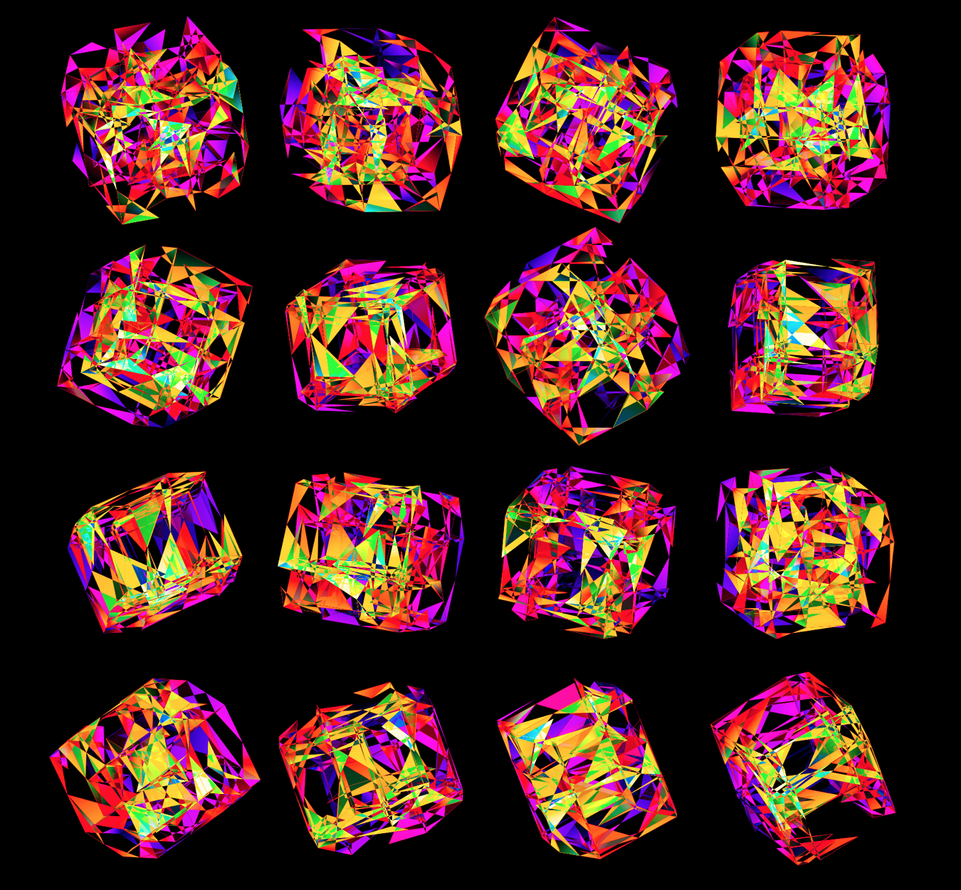
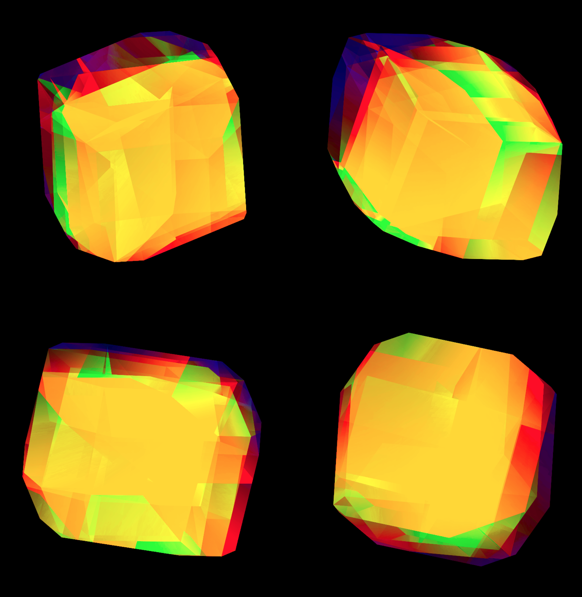
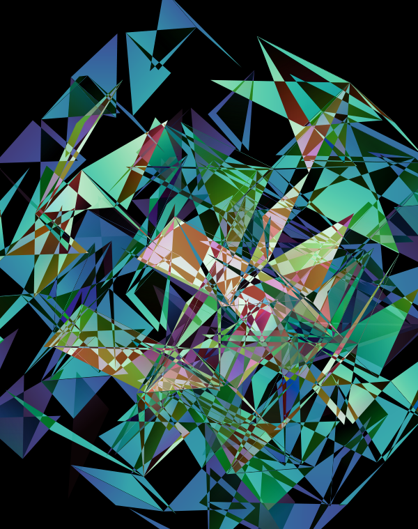
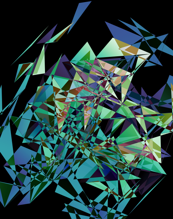
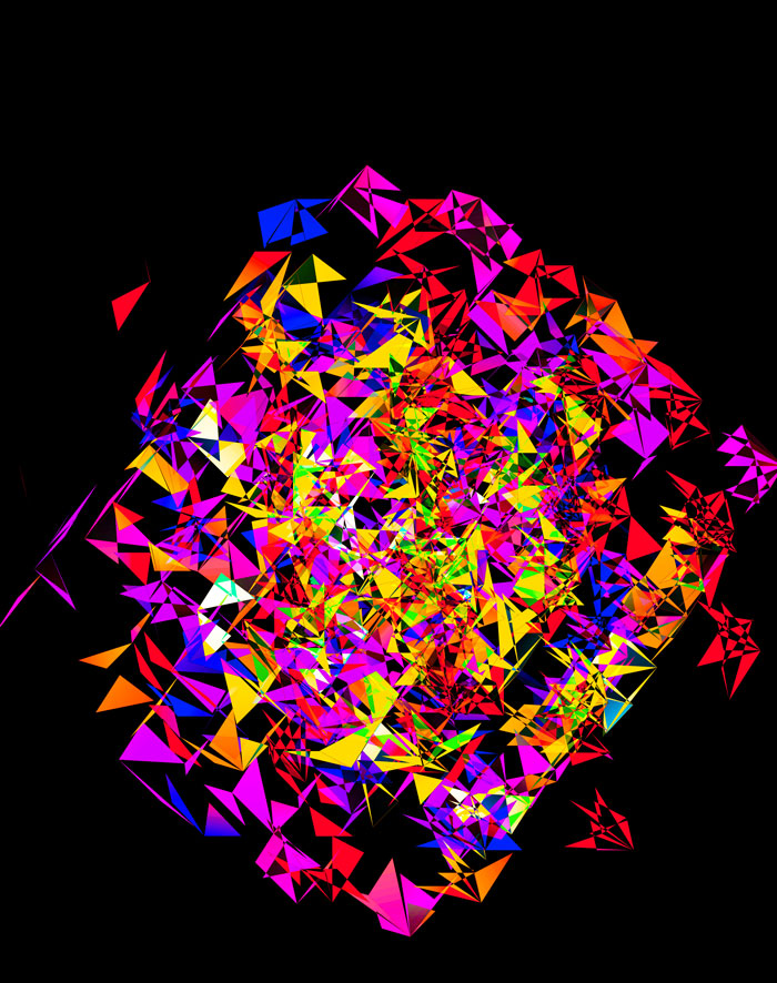
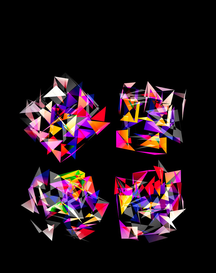
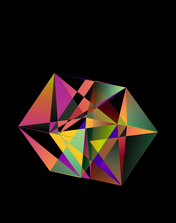
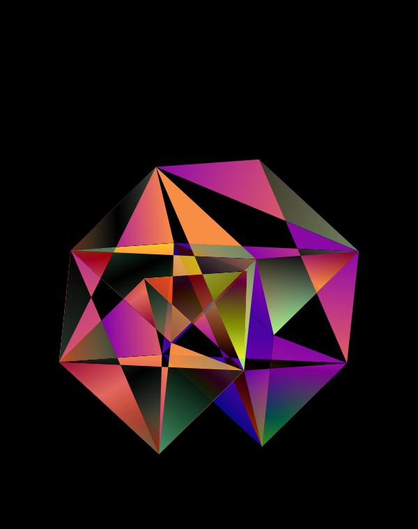
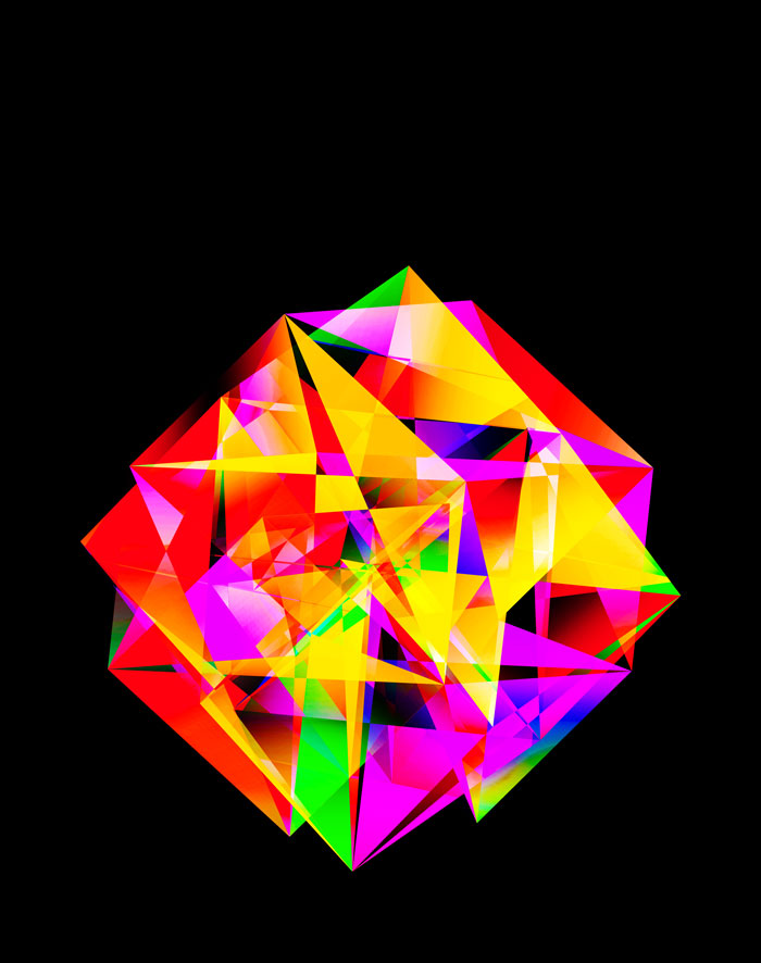
I also experimented with blending two color maps together when the full face was drawn. These don't encode any sequence, but have a very pretty look to them.
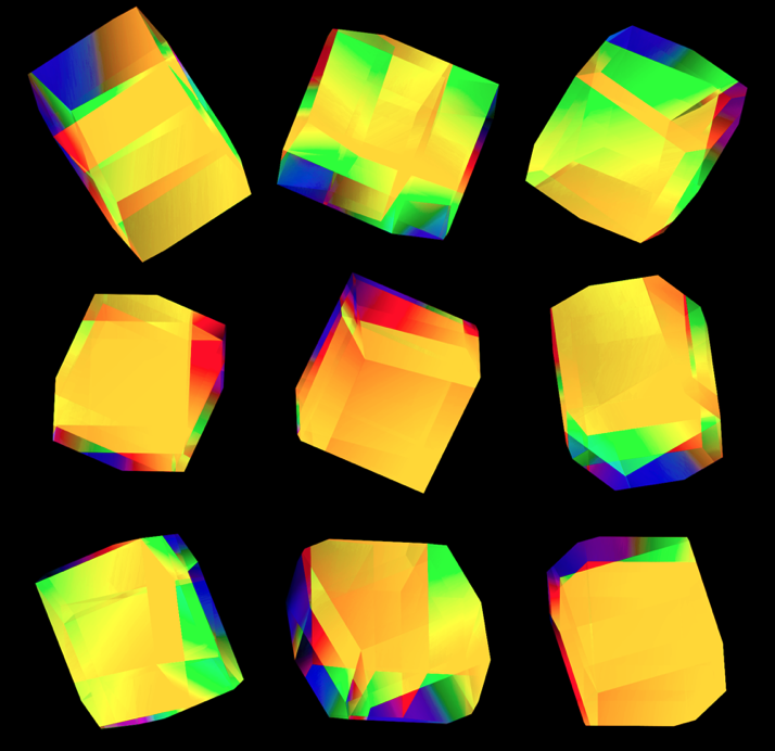
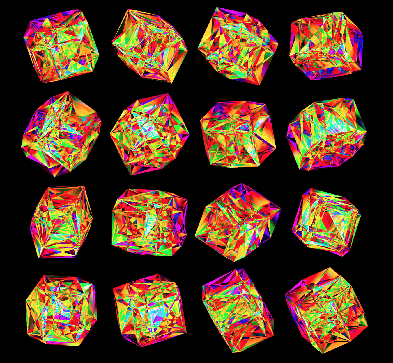
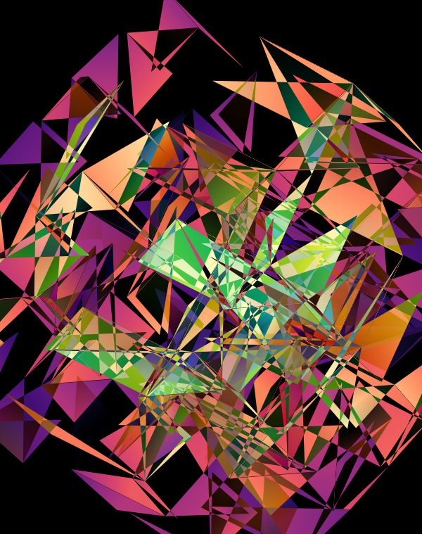
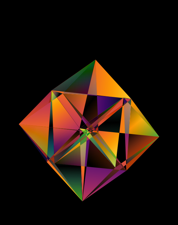
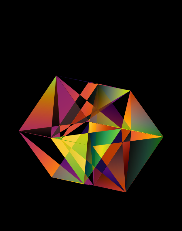
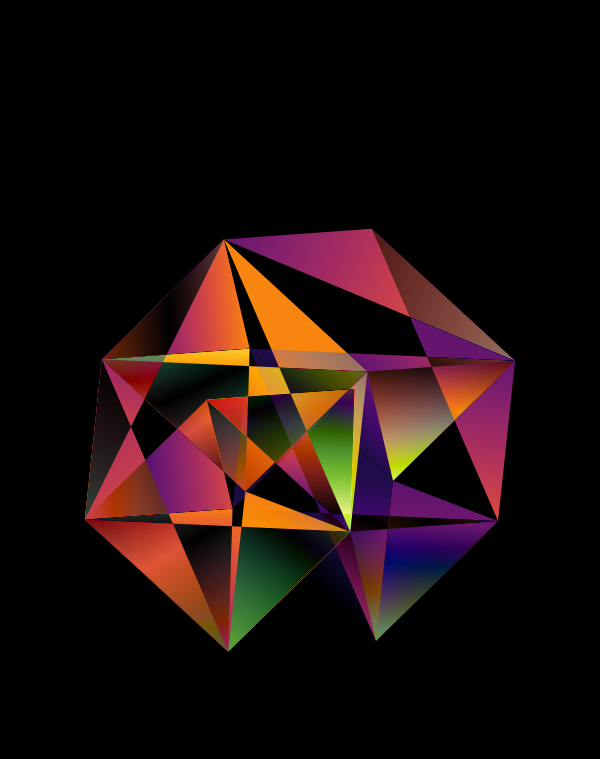
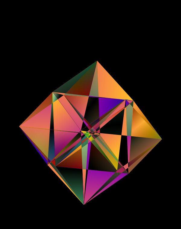
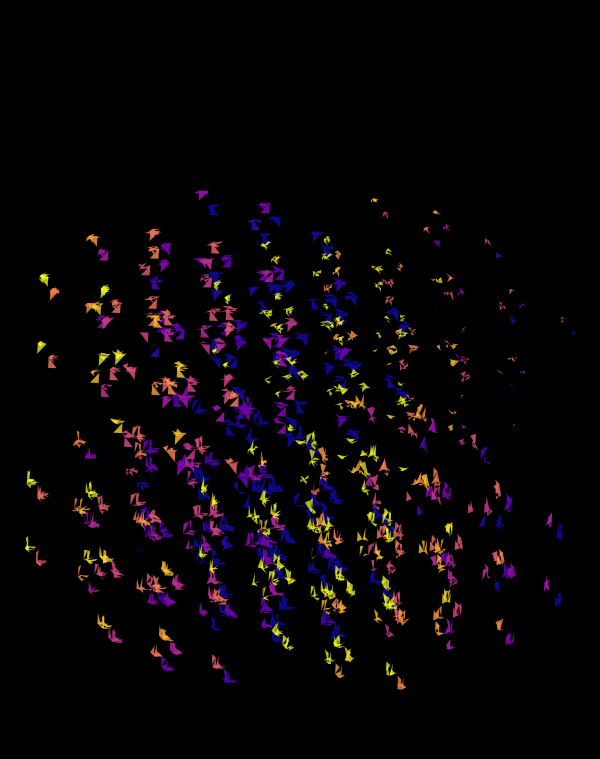
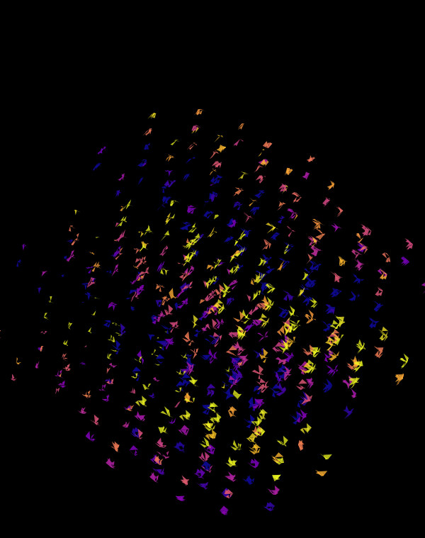
These all look like jewels and at `d=6`, a blend of three cubes, each with a different color map, looks very intriguing. Hhere, I blend three cubes that use viridis, inferno and magma color maps. Magma is very similar to inferno, except it tends more towards the purple at its centre.
Below, I show all individual images from which I made selections for a given version of the final design. There were 6 designs.
For each of the 3 sequence platforms, I tried inferno, plasma, magma, turbo, viridis, mako and white color maps. The inferno, magma and plasma maps are practically identical. For subsequent designs, I won't show images that use the magma or plasma maps.
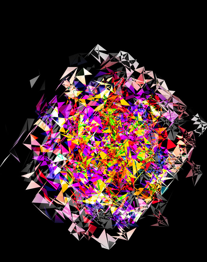
The final designs all show three superimposed cubes, each with its own rotation. Two cubes use a color map and one is drawn with white triangles — blended together with various Photoshop blend modes.
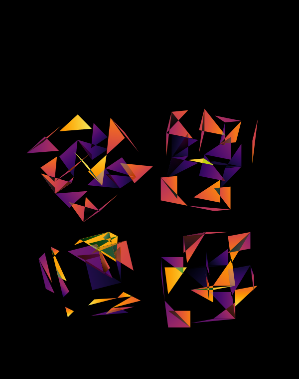
The first design is a close crop of the cubes. Below I show all the images by color map and platform.

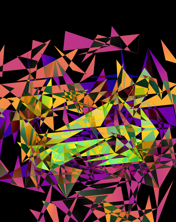
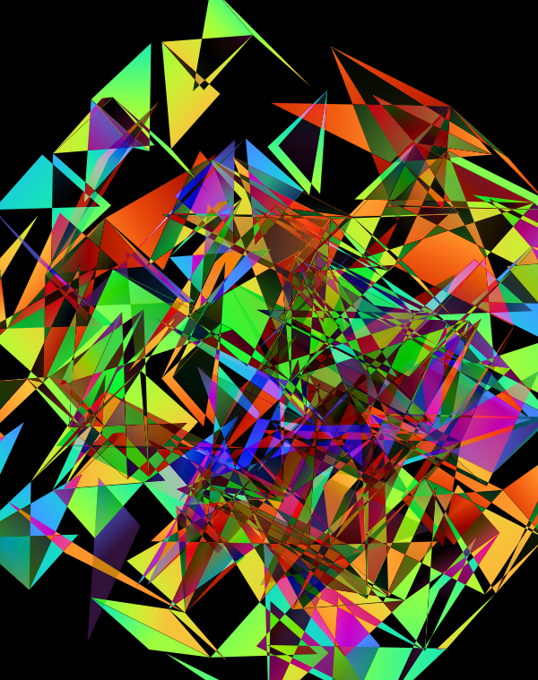
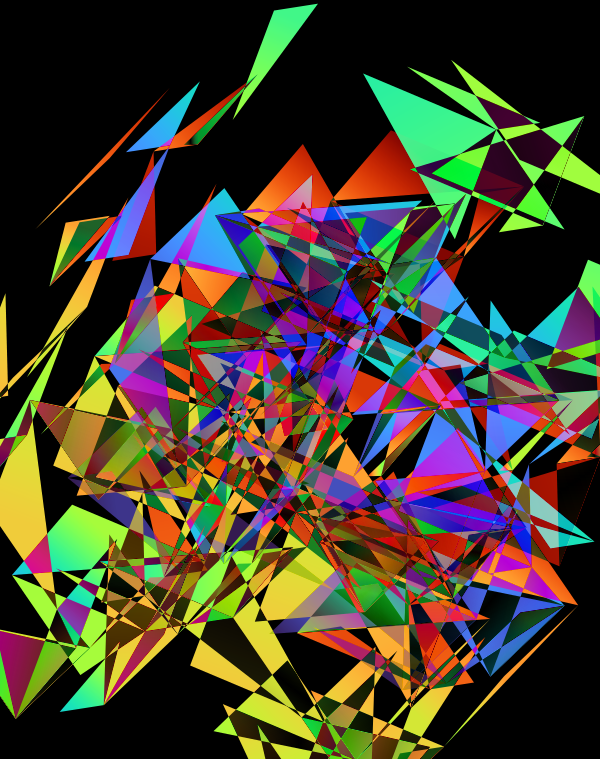
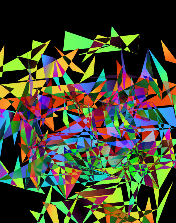
The design used the inferno color maps for 10X and Quartz layers and the white map for the Drop-seq layers. Below, I show how these were blended together.
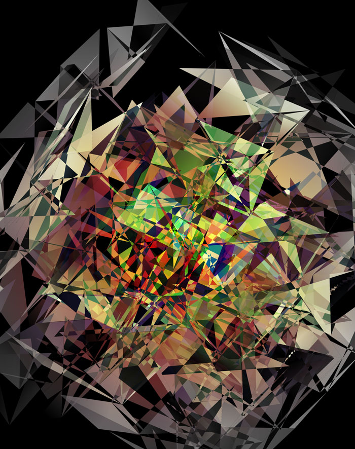
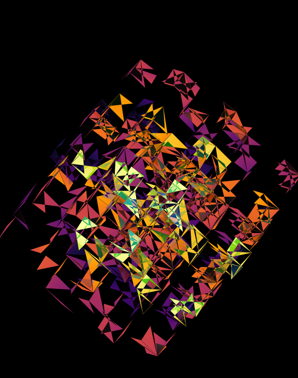
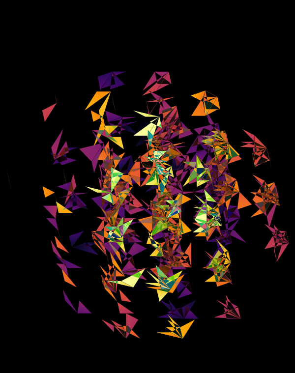
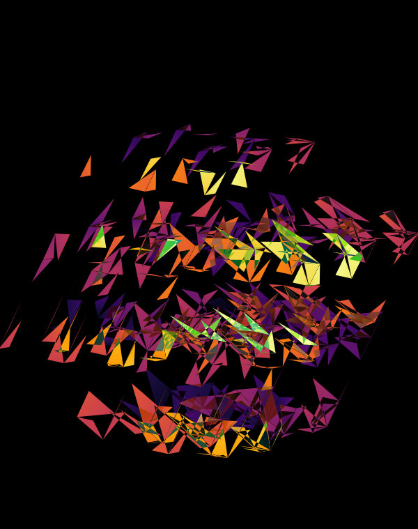
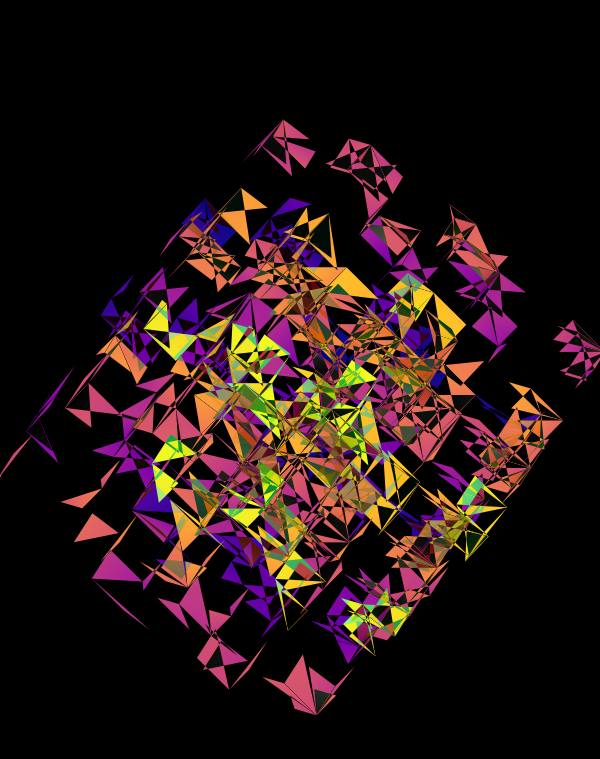
Blending two inferno cubes creates a lot of saturated colors, without a strong sense of depth. The third layer (white, hue blend) very nicely creates a tapering off effect.
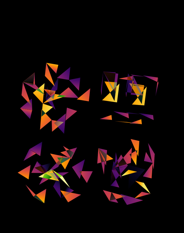
Although this design only uses `d=4` dimensions, it's one of my favourites. It's the only one that shows an array of cubes. In each cell of the array, you see the same set of three cubes (for each of the sequencing platforms) — the only thing that is different is the rotation.
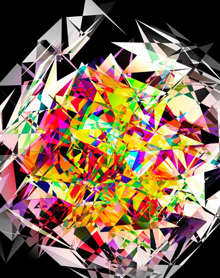
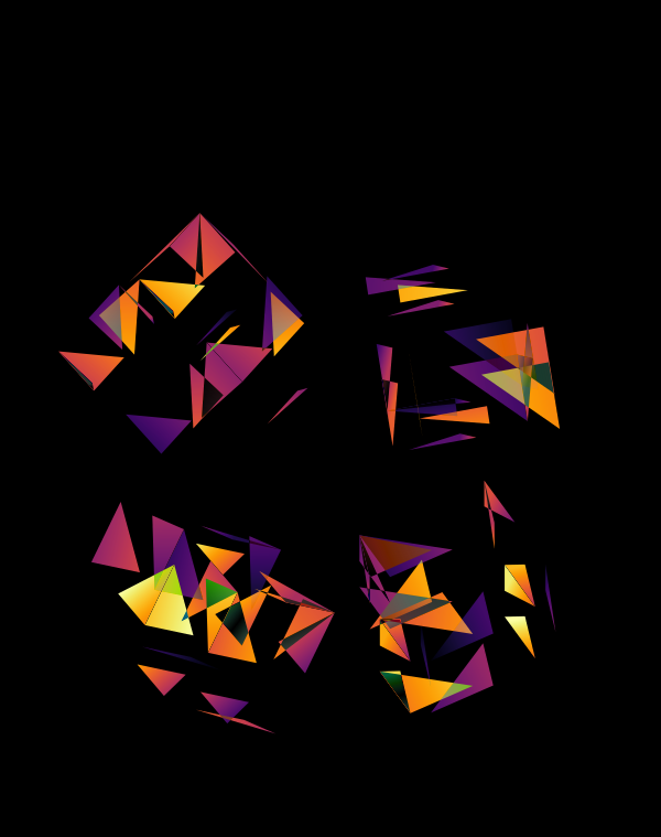
The simplest of all designs — and my favourite. The magic sauce in this design is the soft light blend mode for the second cube.

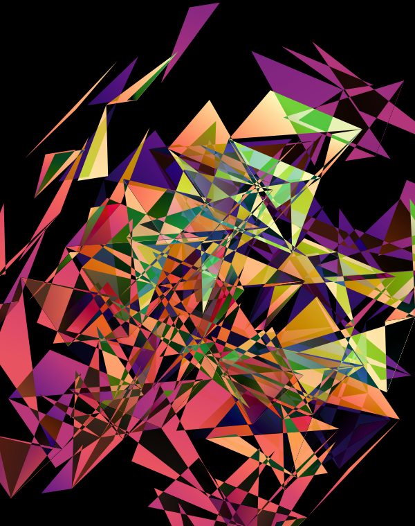
At `d=8` dimensions, each cube has 1,792 faces. In total, there is about 5.3 kb of sequence encoded here.
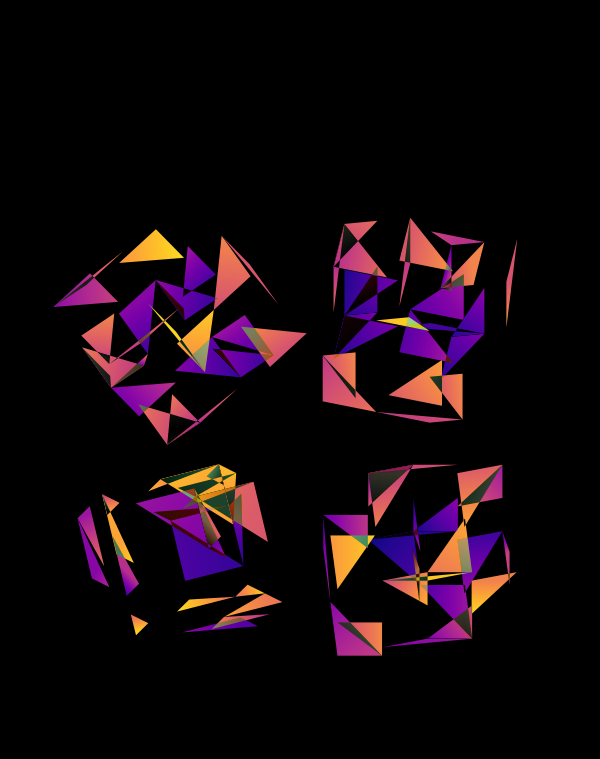
The last design pushes to `d=9` dimensions, where now a cube has 4,608 faces.
Nasa to send our human genome discs to the Moon
We'd like to say a ‘cosmic hello’: mathematics, culture, palaeontology, art and science, and ... human genomes.

Comparing classifier performance with baselines
All animals are equal, but some animals are more equal than others. —George Orwell
This month, we will illustrate the importance of establishing a baseline performance level.
Baselines are typically generated independently for each dataset using very simple models. Their role is to set the minimum level of acceptable performance and help with comparing relative improvements in performance of other models.
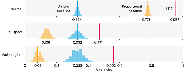
Unfortunately, baselines are often overlooked and, in the presence of a class imbalance5, must be established with care.
Megahed, F.M, Chen, Y-J., Jones-Farmer, A., Rigdon, S.E., Krzywinski, M. & Altman, N. (2024) Points of significance: Comparing classifier performance with baselines. Nat. Methods 20.
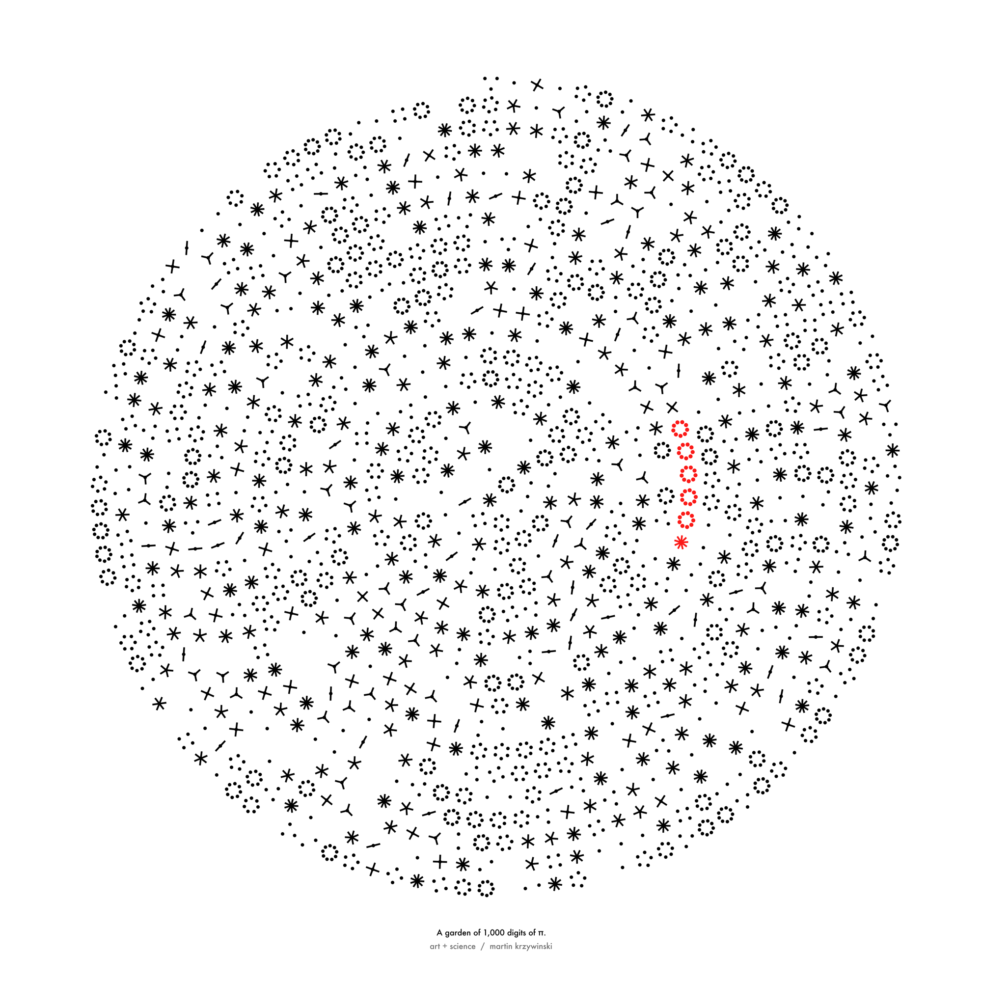
Happy 2024 π Day—
sunflowers ho!
Celebrate π Day (March 14th) and dig into the digit garden. Let's grow something.
How Analyzing Cosmic Nothing Might Explain Everything
Huge empty areas of the universe called voids could help solve the greatest mysteries in the cosmos.
My graphic accompanying How Analyzing Cosmic Nothing Might Explain Everything in the January 2024 issue of Scientific American depicts the entire Universe in a two-page spread — full of nothing.
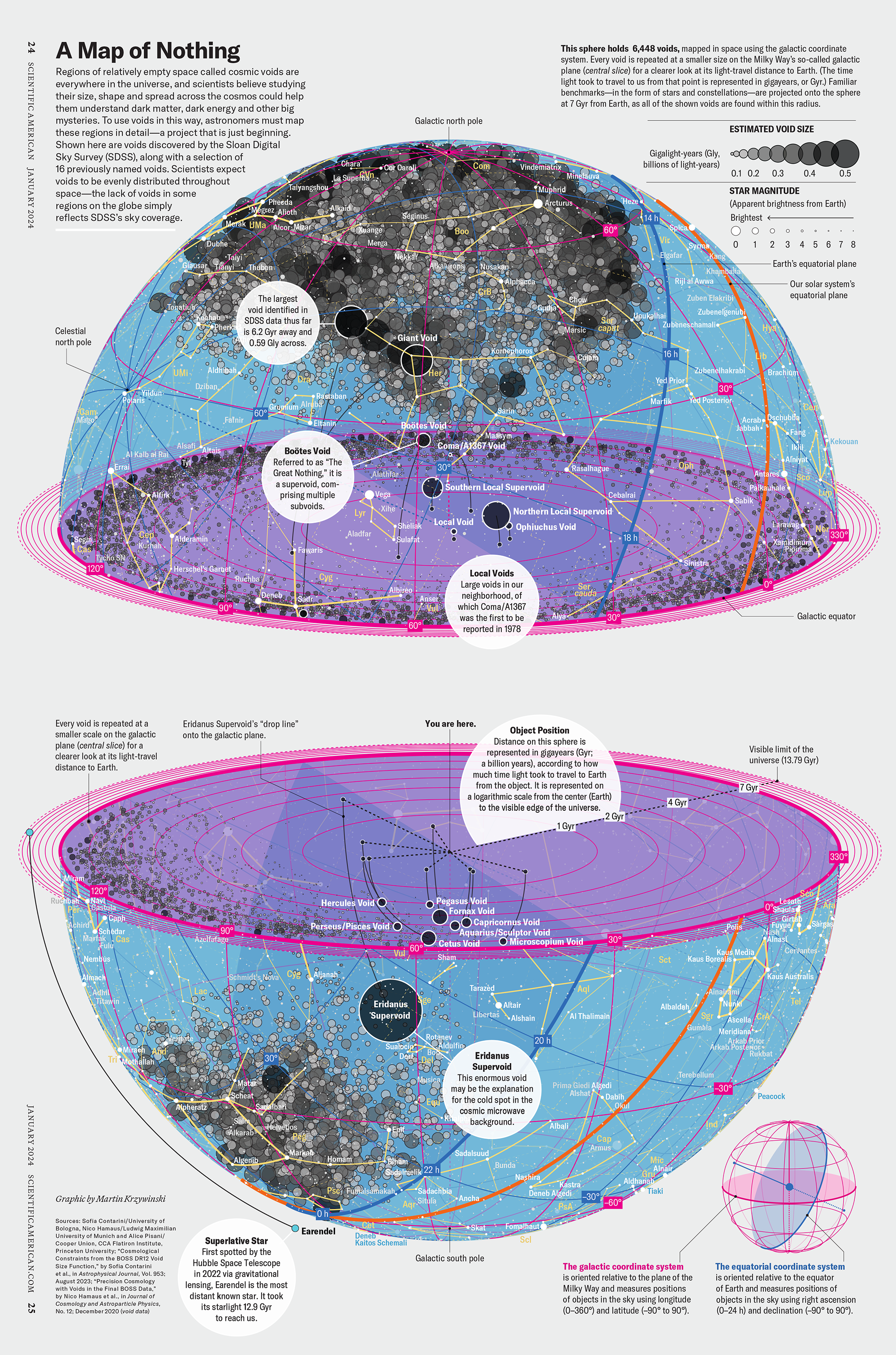
The graphic uses the latest data from SDSS 12 and is an update to my Superclusters and Voids poster.
Michael Lemonick (editor) explains on the graphic:
“Regions of relatively empty space called cosmic voids are everywhere in the universe, and scientists believe studying their size, shape and spread across the cosmos could help them understand dark matter, dark energy and other big mysteries.
To use voids in this way, astronomers must map these regions in detail—a project that is just beginning.
Shown here are voids discovered by the Sloan Digital Sky Survey (SDSS), along with a selection of 16 previously named voids. Scientists expect voids to be evenly distributed throughout space—the lack of voids in some regions on the globe simply reflects SDSS’s sky coverage.”
voids
Sofia Contarini, Alice Pisani, Nico Hamaus, Federico Marulli Lauro Moscardini & Marco Baldi (2023) Cosmological Constraints from the BOSS DR12 Void Size Function Astrophysical Journal 953:46.
Nico Hamaus, Alice Pisani, Jin-Ah Choi, Guilhem Lavaux, Benjamin D. Wandelt & Jochen Weller (2020) Journal of Cosmology and Astroparticle Physics 2020:023.
Sloan Digital Sky Survey Data Release 12
Alan MacRobert (Sky & Telescope), Paulina Rowicka/Martin Krzywinski (revisions & Microscopium)
Hoffleit & Warren Jr. (1991) The Bright Star Catalog, 5th Revised Edition (Preliminary Version).
H0 = 67.4 km/(Mpc·s), Ωm = 0.315, Ωv = 0.685. Planck collaboration Planck 2018 results. VI. Cosmological parameters (2018).
constellation figures
stars
cosmology
Error in predictor variables
It is the mark of an educated mind to rest satisfied with the degree of precision that the nature of the subject admits and not to seek exactness where only an approximation is possible. —Aristotle
In regression, the predictors are (typically) assumed to have known values that are measured without error.
Practically, however, predictors are often measured with error. This has a profound (but predictable) effect on the estimates of relationships among variables – the so-called “error in variables” problem.
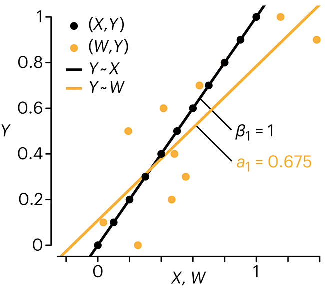
Error in measuring the predictors is often ignored. In this column, we discuss when ignoring this error is harmless and when it can lead to large bias that can leads us to miss important effects.
Altman, N. & Krzywinski, M. (2024) Points of significance: Error in predictor variables. Nat. Methods 20.
Background reading
Altman, N. & Krzywinski, M. (2015) Points of significance: Simple linear regression. Nat. Methods 12:999–1000.
Lever, J., Krzywinski, M. & Altman, N. (2016) Points of significance: Logistic regression. Nat. Methods 13:541–542 (2016).
Das, K., Krzywinski, M. & Altman, N. (2019) Points of significance: Quantile regression. Nat. Methods 16:451–452.