

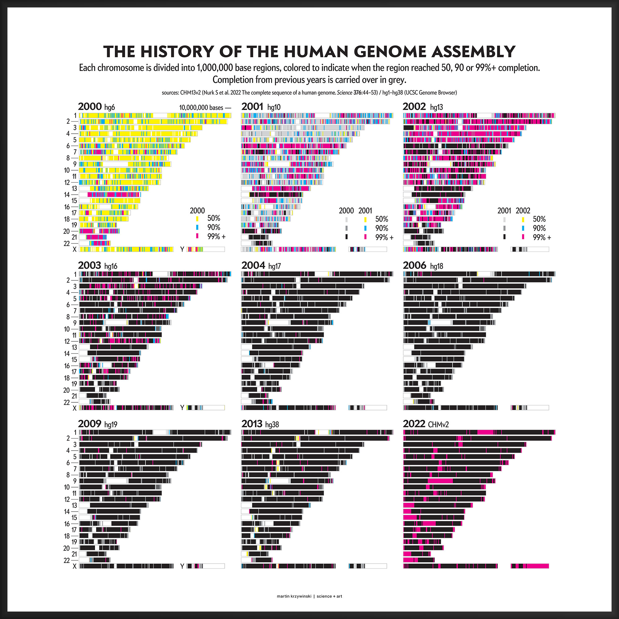
History of the Human Genome Assembly
22 years, 3,117,275,501 bases and 0 gaps later
Round numbers are always false.
— Samuel Johnson
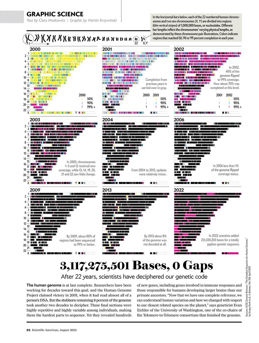
Here, you can expect to learn about the history of the human genome assembly (and a little bit about its structure) and see a map of its completion over the last 22 years, which was published in Scientific American Graphic Science.

contents
In March 2022, a flurry of publications announced the first ever complete assembly of a human genome. This is a big deal because, in genomics, we don't throw around words like “complete” very often. Actually, never — until now.
Because the human genome — a human genome — is complete. All hail the CHM13v2 (Mar 2022) telomere-to-telomere (T2T) assembly.
You've probably already heard — and have been hearing for the last 15 years — that the human genome has been sequenced. After all, how else can there be a publication with the title Finishing the euchromatic sequence of the human genome (2004 Nature 431:931–945).
In 2004, the only thing that stood between “finished” and “complete” was that pesky word “euchromatic”.
“Euchromatin is a lightly packed form of chromatin (DNA, RNA, and protein) that is enriched in genes, and is often (but not always) under active transcription. Euchromatin stands in contrast to heterochromatin, which is tightly packed and less accessible for transcription. 92% of the human genome is euchromatic.” — Wikipedia
For modeling and analysis — such as in cancer research, for example, which is what we do here — by far the most important parts of the human genome assembly are the parts that code for protein (transcribed regions and their ORFs), along with their adjacent regulatory sequences.
These regions in total occupy less than half of the genome. The parts that ultimately translated into protein exons account for just 2.58% of the genome. For the vast majority of genes, the sequence in these regions was indeed finished.

In the most recent assembly prior to the complete telomere-to-telomere CHM13v2 assembly was hg38 (Dec 2013), exons cover only 2.58% of the total sequence (excluding gaps) of the assembly. Notice how much of the open reading frame (ORF) is in introns, which are spliced out during post-transcriptional modification into mature mRNA.
The values in the table above are generated from the size of the union of assembly intervals over the set of genes, because some genes overlap The list of genes includes protein coding, non-coding and pseudogenes.
But with the CHMv2 assembly being more than 200 million bases larger (hello heterochromatin!), we expect to find more genes. And indeed, 3,604 genes, of which 140 are protein coding, are exclusive to CHMv2 (Table 1 in Nurk et al.).
Our goal for the August 2022 Scientific American Graphic Science page was to present the CHMv2 assembly in context of the efforts of the past 22 years — as the final sequencing stage in the sequencing effort. See my other Graphic Science illustrations.
 buy artwork
The DNA samples used to create the reference human sequence assembly used DNA samples from multiple individuals.
The bulk of the genome was sequenced from the RPCI-11 genomic library, which is a collection of about 10,000 randomly sampled pieces (each on average 180,000 bases long) from the genome of an individual male. Other parts of the genome assembly were reconstructed by sequencing RPCI-13 (female) and Caltech-D (Table 2 in Zhao (2000)) libraries.
The human genome is a variable quantity — two individuals vary, on average, by 1 base in 1,000 (or, roughly, in about 3 million positions) — and much of human genomics deals with understanding and handling this variability.
As such, the term “the human genome” is a little misleading and it's important to acknowledge that, given this natural variation between individuals (and even between cells within an individual), there is really no such thing.
When we say “the genome” we invariably mean “the reference genome”. Even then, we need to specify which version of the reference we mean. At the moment (July 2022), the hg38 (Dec 2013) assembly is considered to be the canonical reference and this may not change anytime soon. It's not uncommon (especially for several months after the release of a new assembly) to find genomic resources that use older references — updating an analysis or data pipeline to a new reference assembly is not a trivial task.
For example, well after the release of hg38 (Dec 2013), the previous reference hg19 (Feb 2009) continued to be widely used for several years. To facilitate standardizing results to the same assembly, so-called liftOver annotations allow conversion of one assembly's coordinates to another.
As the sequence assembly matured, regions were successively filled in by targeted efforts focusing on specific regions (e.g. DNA sequence analysis of human chromosome 9) or by specific institutions (e.g. A Japanese history of the Human Genome Project).
This kind of focused effort to improve the assembly quality of a region was always part of the process. In fact, already in 2000 you can see that significant portions of chromosomes 14, 20, 21 and 22 were completed to 99%+. In 2001, chromosomes 6 and 13 received a lot of attention.
In contrast to focused sequencing, other parts of the assembly were sequenced in a shotgun fashion — by randomly sampling as many regions in the genome as possible in an effort to spread out the coverage. Early on, the shotgun effort was accelerated so that the public assembly would provide more coverage (with commensurately higher quality) than the private sector assembly created by Celera.
Over the years 2000 to 2013, the human genome assembly progressively improved from a so-called “draft” assembly to one that, practically, may be called “finished” (finishish?). These terms can be defined in various ways — for example, based on how much of coding sequence is represented, the contiguity of the assembly, the total coverage of the genome, or some combination of these metrics.
Individual assemblies were indexed by hgN from hg1 (May 2000) to hg38 (Dec 2013). Differences in the index value do not necessarily represent how much of the assembly changed and some indexes were skipped. And I'm still trying to locate the sequence files of hg3 (July 2000).
The hg prefix was used by the team at the UCSC Genome Browser while NCBI had their own assembly build indexes (e.g. hg10 was NCBI build 28). In fact, as of July 2022, there are 1,268 assemblies of the human genome indexed by NCBI.
The hg38 (Dec 2013) assembly continues to be the canonical “reference sequence” since 2013 (and likely beyond 2022). An excellent assembly, it nevertheless contains 1,001 gaps totalling about 150 Mb across chromosomes 1–22, X and Y. as well as 430 unanchored and alternate pieces that totalled 121 Mb and themselves include 240 gaps of about 9 Mb.

These gaps were mostly in heterochromatic regions, which are notoriously difficult to sequence. When the size of the gap was not known, following tradition, it was set to 100 bases . Other sizes, such as 1kb, 10kb and 50kb signalled more information about the nature of the gap, such as a contig gap, short arm gap, telomere gap, and so on.
The CHM13v2 (Mar 2022) assembly filled in all these gaps. It is a completely gapless assembly.
Propensity score weighting
The needs of the many outweigh the needs of the few. —Mr. Spock (Star Trek II)
This month, we explore a related and powerful technique to address bias: propensity score weighting (PSW), which applies weights to each subject instead of matching (or discarding) them.
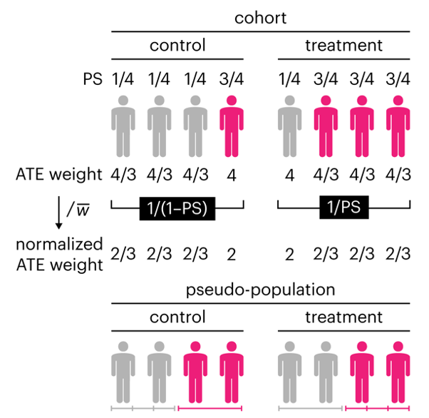
Kurz, C.F., Krzywinski, M. & Altman, N. (2025) Points of significance: Propensity score weighting. Nat. Methods 22:1–3.
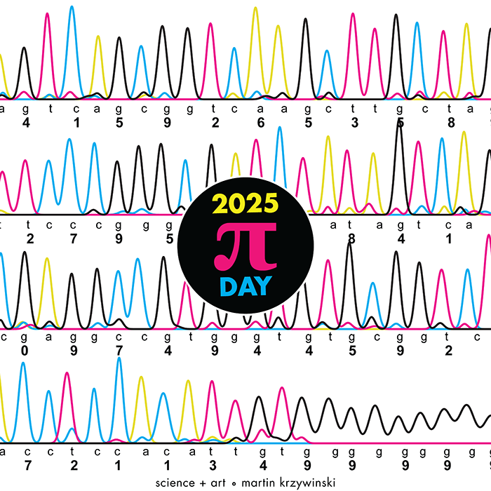
Happy 2025 π Day—
TTCAGT: a sequence of digits
Celebrate π Day (March 14th) and sequence digits like its 1999. Let's call some peaks.
Crafting 10 Years of Statistics Explanations: Points of Significance
I don’t have good luck in the match points. —Rafael Nadal, Spanish tennis player
Points of Significance is an ongoing series of short articles about statistics in Nature Methods that started in 2013. Its aim is to provide clear explanations of essential concepts in statistics for a nonspecialist audience. The articles favor heuristic explanations and make extensive use of simulated examples and graphical explanations, while maintaining mathematical rigor.
Topics range from basic, but often misunderstood, such as uncertainty and P-values, to relatively advanced, but often neglected, such as the error-in-variables problem and the curse of dimensionality. More recent articles have focused on timely topics such as modeling of epidemics, machine learning, and neural networks.
In this article, we discuss the evolution of topics and details behind some of the story arcs, our approach to crafting statistical explanations and narratives, and our use of figures and numerical simulations as props for building understanding.
Altman, N. & Krzywinski, M. (2025) Crafting 10 Years of Statistics Explanations: Points of Significance. Annual Review of Statistics and Its Application 12:69–87.
Propensity score matching
I don’t have good luck in the match points. —Rafael Nadal, Spanish tennis player
In many experimental designs, we need to keep in mind the possibility of confounding variables, which may give rise to bias in the estimate of the treatment effect.
If the control and experimental groups aren't matched (or, roughly, similar enough), this bias can arise.
Sometimes this can be dealt with by randomizing, which on average can balance this effect out. When randomization is not possible, propensity score matching is an excellent strategy to match control and experimental groups.
Kurz, C.F., Krzywinski, M. & Altman, N. (2024) Points of significance: Propensity score matching. Nat. Methods 21:1770–1772.
Understanding p-values and significance
P-values combined with estimates of effect size are used to assess the importance of experimental results. However, their interpretation can be invalidated by selection bias when testing multiple hypotheses, fitting multiple models or even informally selecting results that seem interesting after observing the data.
We offer an introduction to principled uses of p-values (targeted at the non-specialist) and identify questionable practices to be avoided.
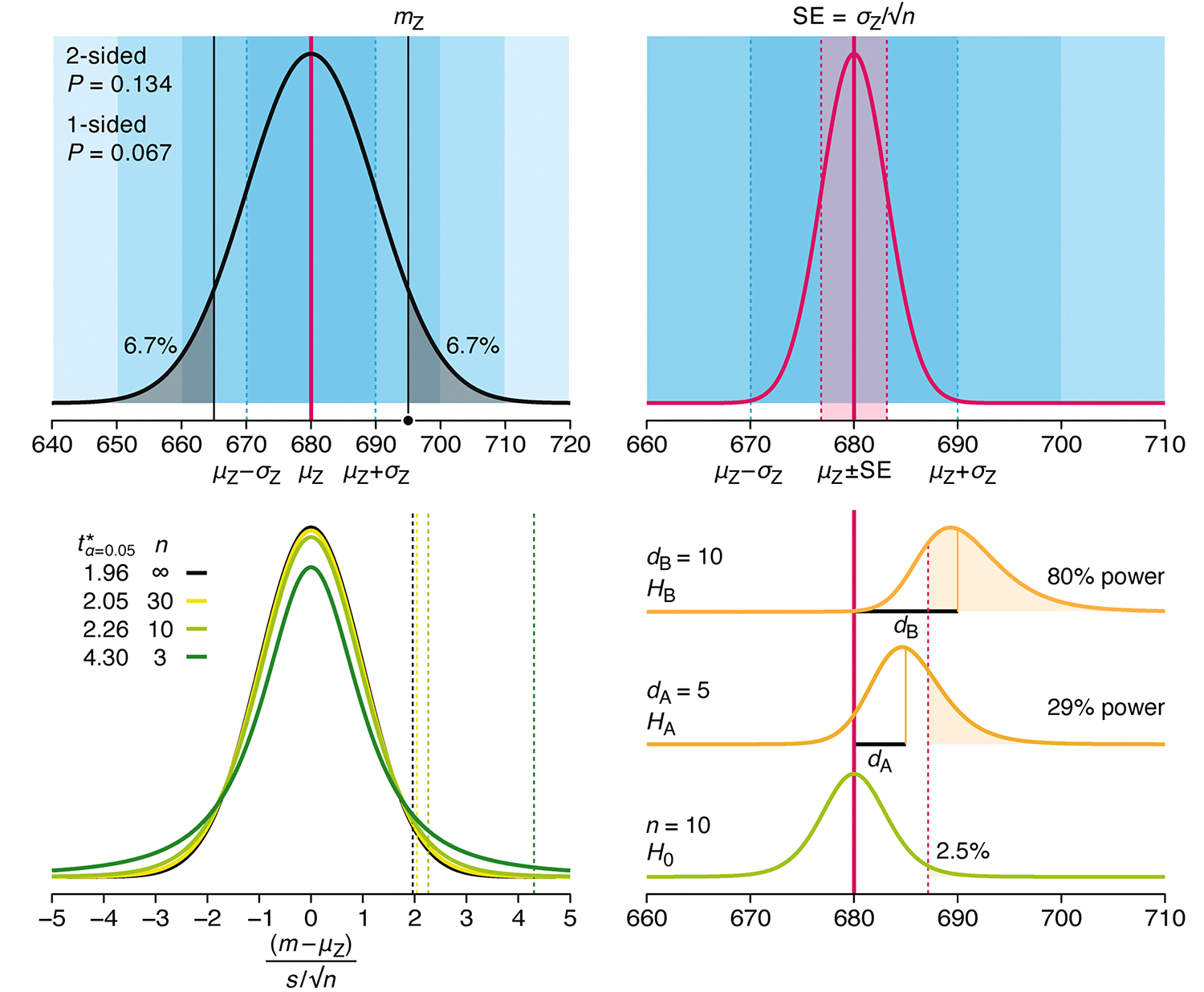
Altman, N. & Krzywinski, M. (2024) Understanding p-values and significance. Laboratory Animals 58:443–446.