
 buy artwork
`\pi` Approximation Day Art Posters


The never-repeating digits of `\pi` can be approximated by 22/7 = 3.142857 to within 0.04%. These pages artistically and mathematically explore rational approximations to `\pi`. This 22/7 ratio is celebrated each year on July 22nd. If you like hand waving or back-of-envelope mathematics, this day is for you: `\pi` approximation day!
Equip your imagination.
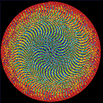
What would circles look like if `\pi`=22/7?
Tiny loop, Folded dimensions and solidland
Imagine that the circle had a tiny loop at one of its points. The circumference of this loop would be added to the circumference of the circle, but the loop would be so small that we would never notice it.

This is reminiscent of how string theories describe higher dimensions—as tiny loops at each point in space, except in my example the loop is only at one point.

This idea originated with Klein, who explained the fourth dimension as a curled up circle of a very small radius. Another way in which this curling-up is used is to say that the fifth dimension is a curled up Planck length, as explained in this Imagining 10 Dimensions video.
flatlanders and solidlanders
If this idea is difficult to wrap your head around, you're not alone. We cannot think of additional dimensions in the regular spatial sence since we have no means of experiencing such phenomena. We can however imagine how flatlanders might explain the 3rd dimension, since we can perceive it. They would draw the curled up circles in their plane because they would not have the experience of drawing with perspective mimicking our 3rd dimension.

We would draw their explanation as shown on the right in the figure above, borrowing from our concept of the 3rd spatial dimension. Now imagine showing our explanation to a flatlander. They would not see the same thing as you—the circles would not intuitively imply the higher dimension to them.
This is analogous to why we cannot draw folded up dimensions. We are merely solidlanders—flatlanders in 3d space. Creatures that can perceive more spatial dimensions would use us as examples of diminished perceptual ability.
relativistic speeds, frames of reference and length contraction
Another way to imagine how a circle might look is a little more realistic. The theory of special relativity tells us that when we travel at speed relative to another object the dimensions of that object appear contracted to us in the direction of motion.
This contraction is always present, but essentially imperceptible unless we're travelling fast enough. For example, in order for a 1 meter object to appear contracted by the length of a hydrogen molecule (0.3 nm) we would have to be travelling at 7.3 km/s (Wolfram Alpha calculation)!

How fast would we have to be going to compress the circle sufficiently so that its circumference and radius ratio embody the `22/7` approximation of `\pi`? Pretty fast, it turns out. If we travel at just over 12,000 km/sec (0.04 times the speed of light, Wolfram Alpha calculation), the circle will compress as shown in the figure above, and the ratio of its circumference to the radius along direction of motion will make `\pi` appear to be `22/7`.
This compression in length would be barely perceptible to us. Below are both circles, shown overlapping, with `delta` being the extra length in radius required.

The value of `\delta`, which is 0.0008049179155 (if `r = 1`), can be calculated by considering the perimeter of an ellipse. The fact that `\delta` is small shouldn't be surprising since `22/7` is an excellent approximation of `\pi`, good to 0.04%.
Calculating the parameter of an ellipse is more complicated than calculating it for a circle because it uses something called an elliptic integral. This integral has no analytical solution and requires numerical approximation. Luckily, we have computers.

We can use the expression shown above for the perimeter of the ellipse to determine how much the circle needs to be deformed. Let's write `a = r + \delta` (original radius with slight deformation `\delta`) and `b=r`. Since `22/7 > \pi` we know that `\delta > 0`.
It remains to solve the equation below for a value of `\delta` that will yield a ratio of circumference to `r` of `2 \times 22/7`.

To make things simpler, let set `r=1`. Solving the equation numerically, I find $$\delta = 0.0008049179155$$
You can verify this solution at Wolfram Alpha.
the meaning of full-circle
After all this, we come full-circle to the meaning of full-circle.
You might ask why I didn't change the definition of `\pi` to `22/7` in the upper limit of the integral. After all, why not make the approximation exercise more faithful to the approximation?
It turns out that if I did that I would get `\delta=0`, which brings us back to the original circle. How is this possible?
Technically, this is because the integral returns the upper limit as its answer if the eccentricity is zero (i.e., `E(x,0)=x`).
Intuitively, this is because changing the upper limit of the integral actually redefines the angle of a full revolution. Now, full-circle isn't `2 \pi` radians, but `2 \times 22/7`. Given that the ratio of the circumference of a circle to its radius is exactly the size, in radians, of a full revolution, we don't need to change the shape of the circle if we're willing to change what a full revolution means.
Beyond Belief Campaign BRCA Art
Fuelled by philanthropy, findings into the workings of BRCA1 and BRCA2 genes have led to groundbreaking research and lifesaving innovations to care for families facing cancer.
This set of 100 one-of-a-kind prints explore the structure of these genes. Each artwork is unique — if you put them all together, you get the full sequence of the BRCA1 and BRCA2 proteins.

Propensity score weighting
The needs of the many outweigh the needs of the few. —Mr. Spock (Star Trek II)
This month, we explore a related and powerful technique to address bias: propensity score weighting (PSW), which applies weights to each subject instead of matching (or discarding) them.
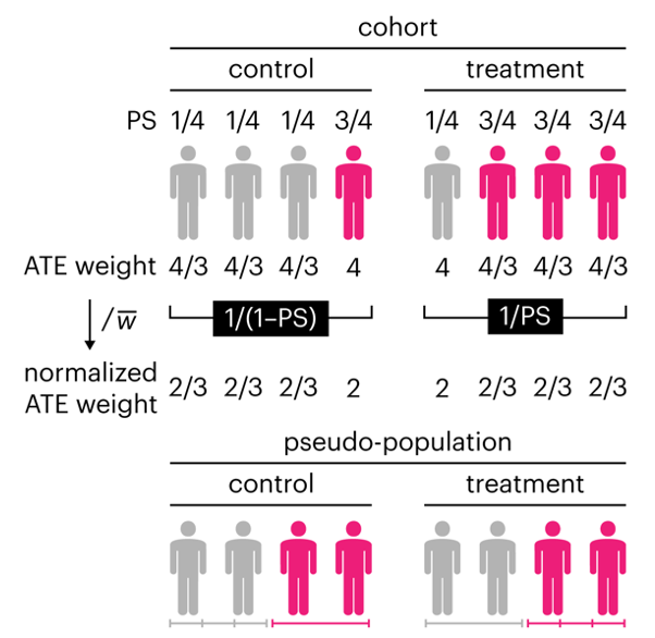
Kurz, C.F., Krzywinski, M. & Altman, N. (2025) Points of significance: Propensity score weighting. Nat. Methods 22:1–3.
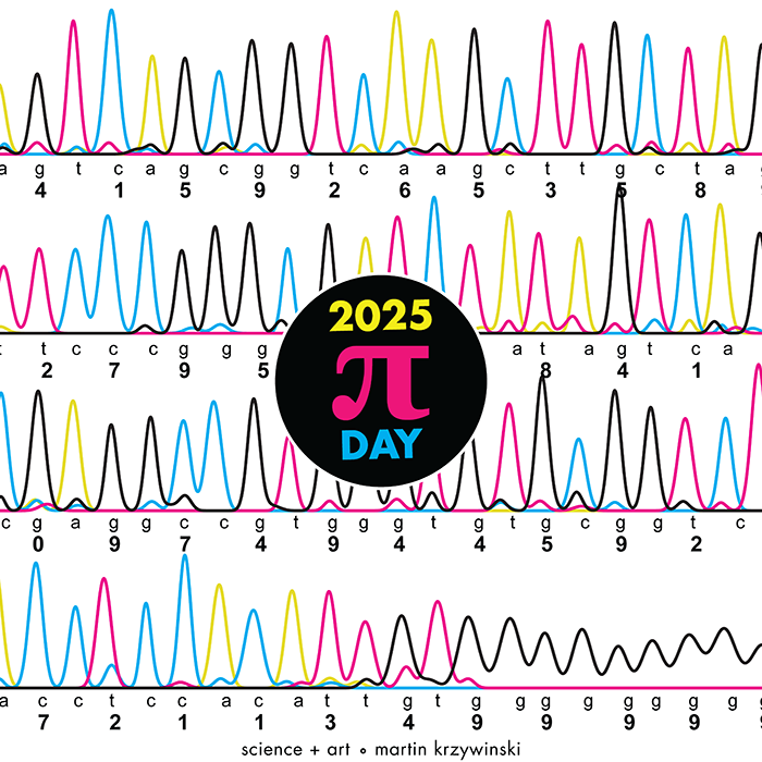
Happy 2025 π Day—
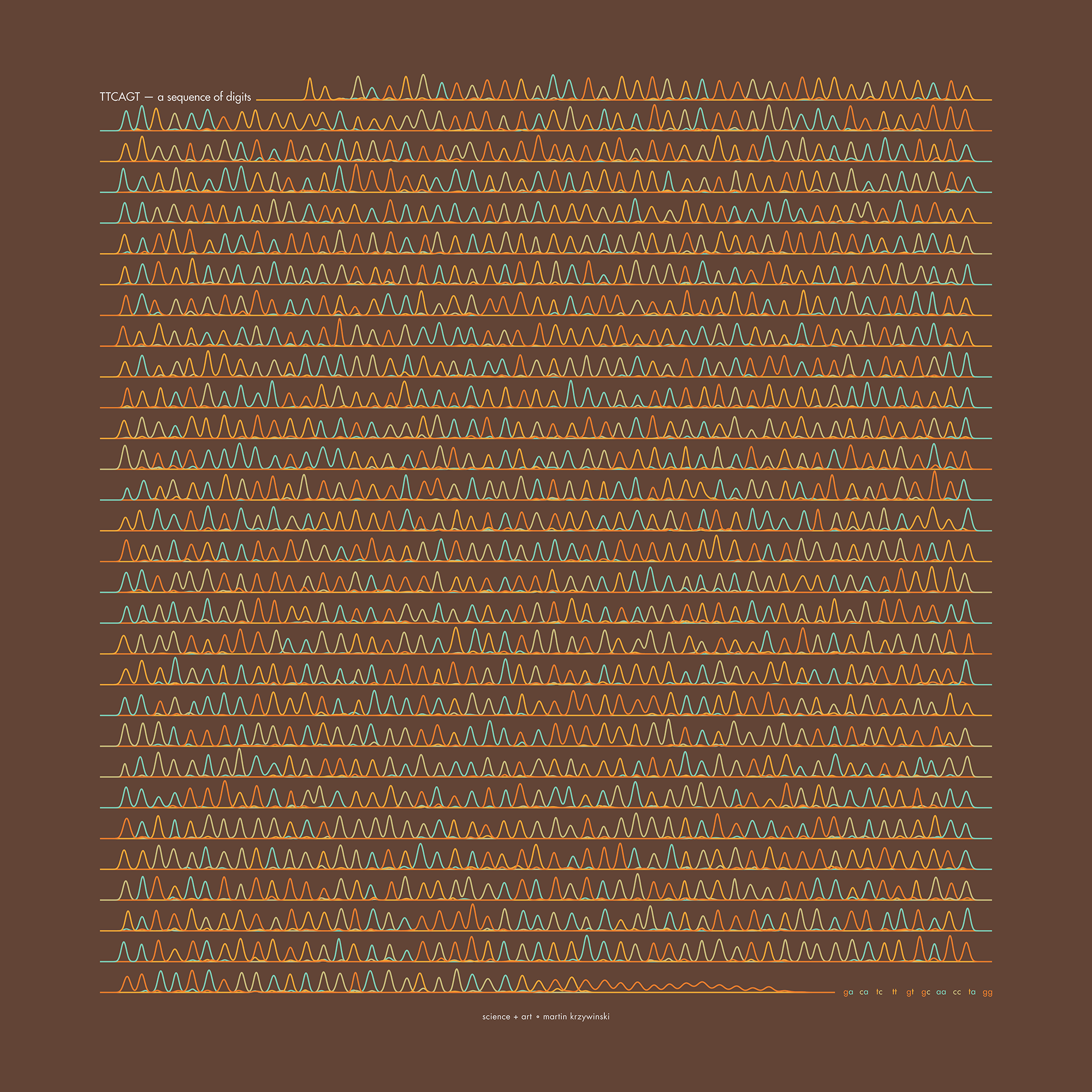
TTCAGT: a sequence of digits
Celebrate π Day (March 14th) and sequence digits like its 1999. Let's call some peaks.
Crafting 10 Years of Statistics Explanations: Points of Significance
I don’t have good luck in the match points. —Rafael Nadal, Spanish tennis player
Points of Significance is an ongoing series of short articles about statistics in Nature Methods that started in 2013. Its aim is to provide clear explanations of essential concepts in statistics for a nonspecialist audience. The articles favor heuristic explanations and make extensive use of simulated examples and graphical explanations, while maintaining mathematical rigor.
Topics range from basic, but often misunderstood, such as uncertainty and P-values, to relatively advanced, but often neglected, such as the error-in-variables problem and the curse of dimensionality. More recent articles have focused on timely topics such as modeling of epidemics, machine learning, and neural networks.
In this article, we discuss the evolution of topics and details behind some of the story arcs, our approach to crafting statistical explanations and narratives, and our use of figures and numerical simulations as props for building understanding.
Altman, N. & Krzywinski, M. (2025) Crafting 10 Years of Statistics Explanations: Points of Significance. Annual Review of Statistics and Its Application 12:69–87.
Propensity score matching
I don’t have good luck in the match points. —Rafael Nadal, Spanish tennis player
In many experimental designs, we need to keep in mind the possibility of confounding variables, which may give rise to bias in the estimate of the treatment effect.
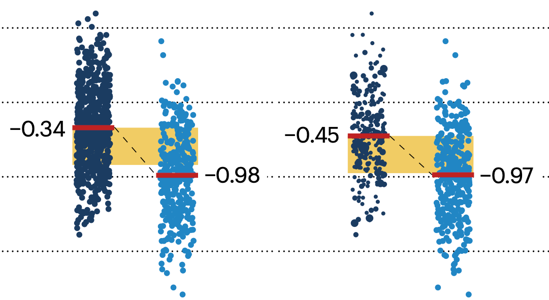
If the control and experimental groups aren't matched (or, roughly, similar enough), this bias can arise.
Sometimes this can be dealt with by randomizing, which on average can balance this effect out. When randomization is not possible, propensity score matching is an excellent strategy to match control and experimental groups.
Kurz, C.F., Krzywinski, M. & Altman, N. (2024) Points of significance: Propensity score matching. Nat. Methods 21:1770–1772.
Understanding p-values and significance
P-values combined with estimates of effect size are used to assess the importance of experimental results. However, their interpretation can be invalidated by selection bias when testing multiple hypotheses, fitting multiple models or even informally selecting results that seem interesting after observing the data.
We offer an introduction to principled uses of p-values (targeted at the non-specialist) and identify questionable practices to be avoided.
Altman, N. & Krzywinski, M. (2024) Understanding p-values and significance. Laboratory Animals 58:443–446.