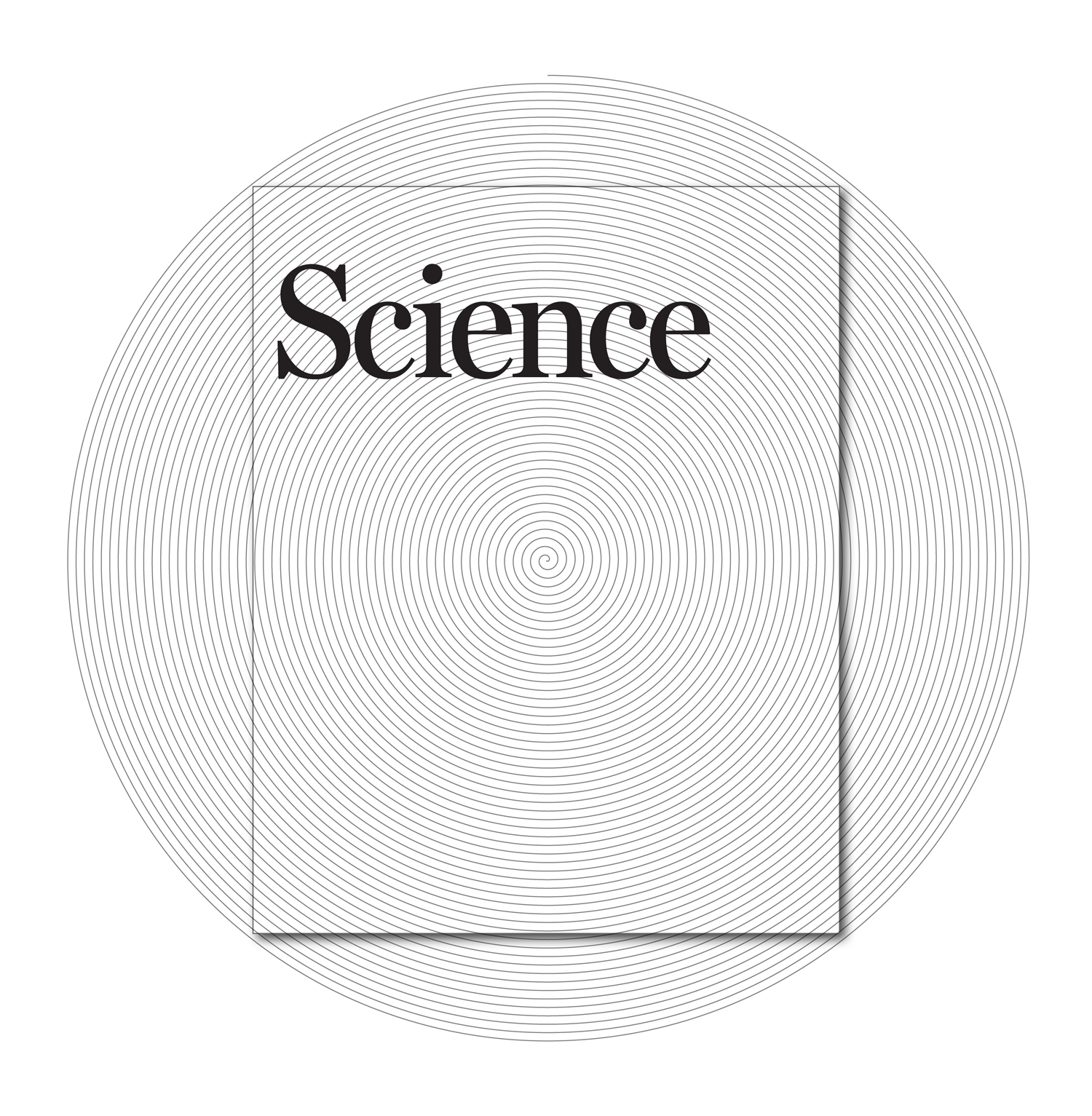
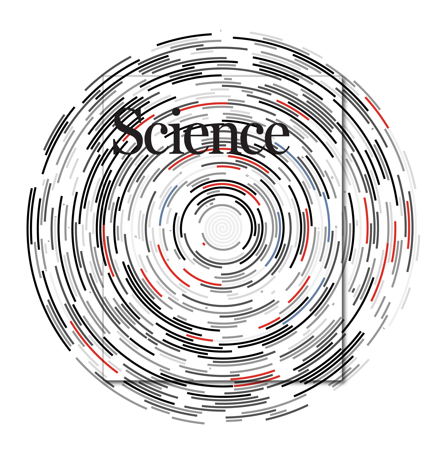
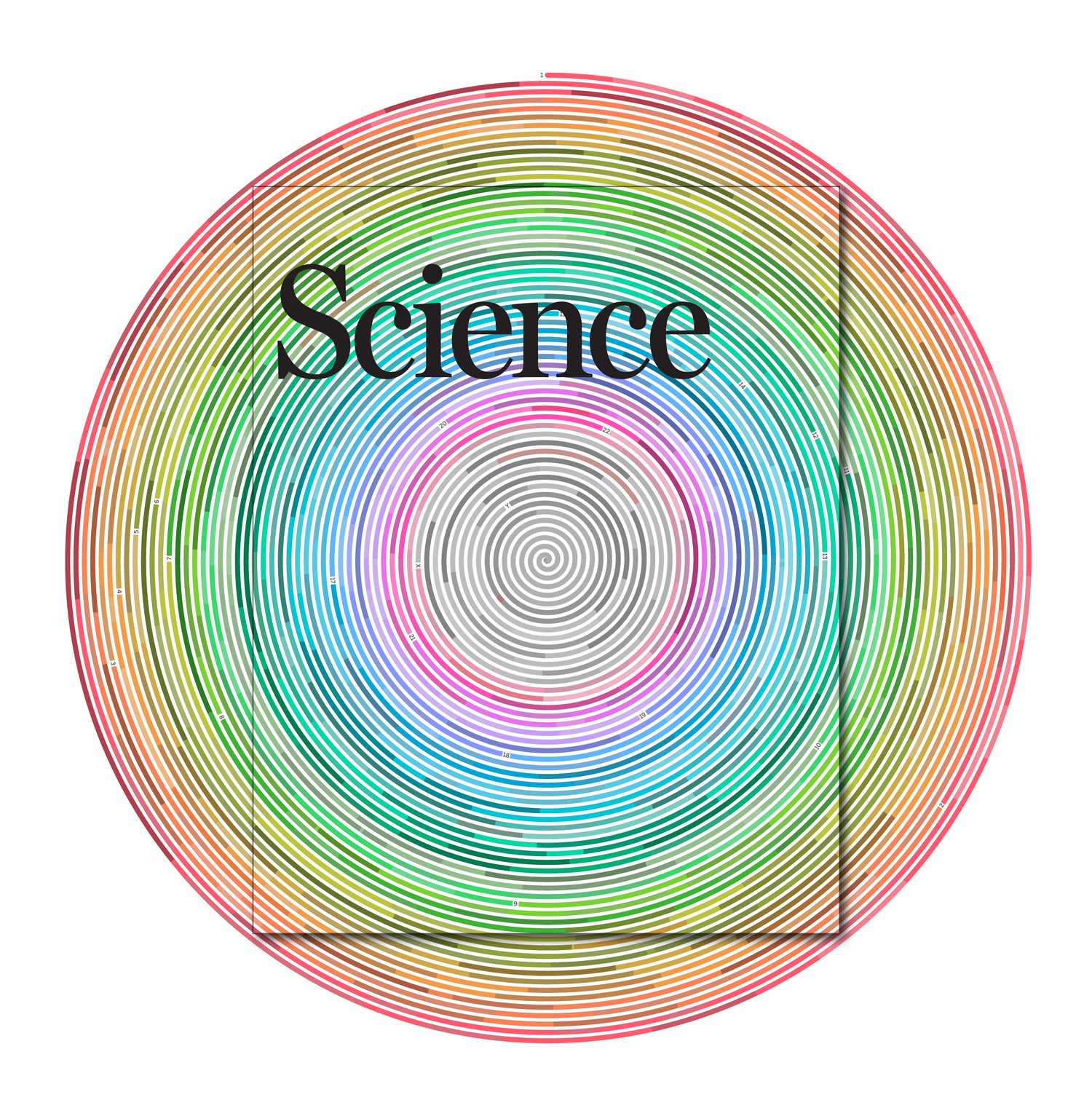
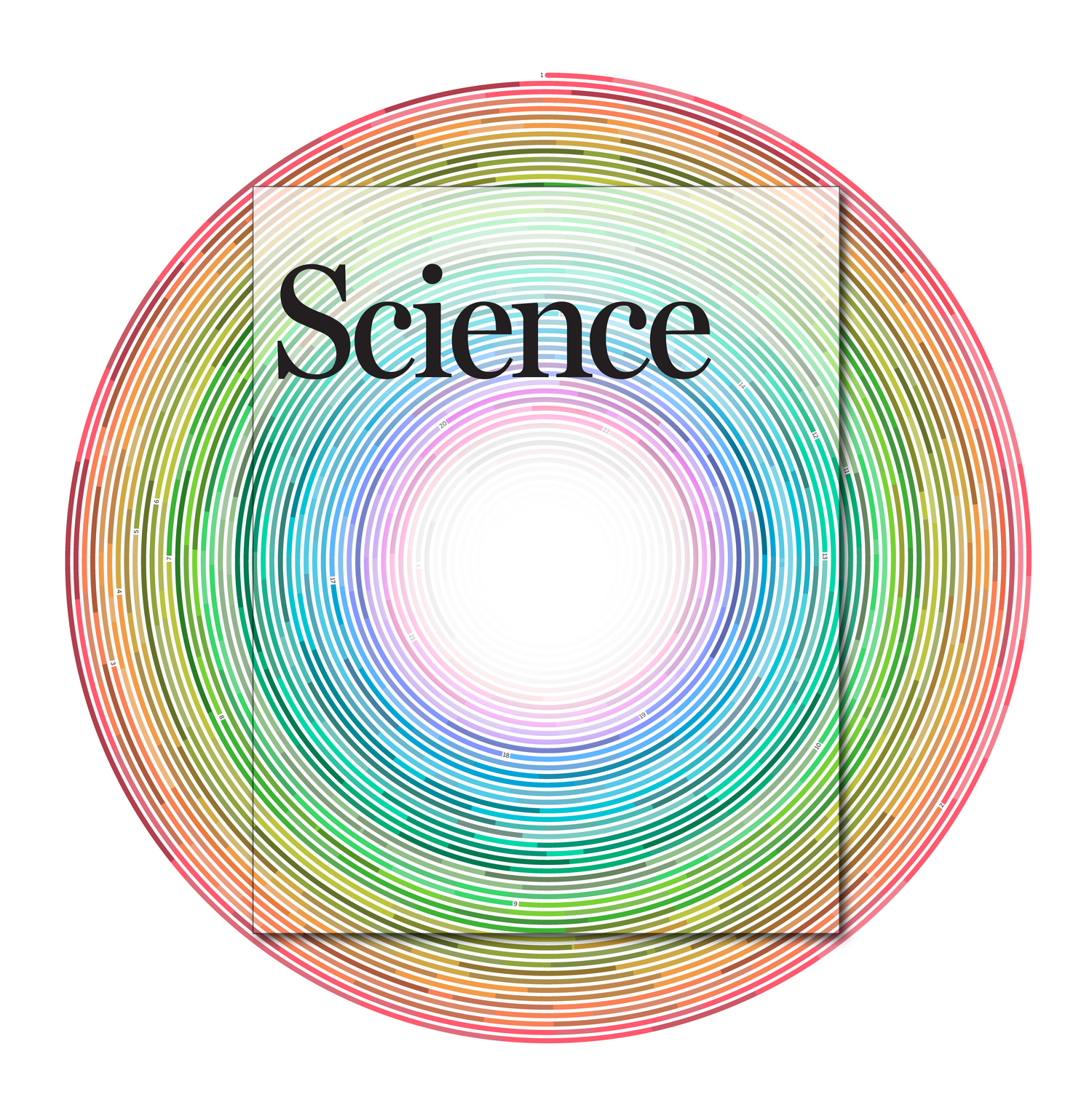
Science Magazine cover — Human Genome Special Issue
The issue explores lessons from past studies of human genomics, with an eye toward future research efforts | 24 September 2021 | Volume 373 | Issue 6562
data sources
1. Amberger JS, Bocchini CA, Schiettecatte FJM, Scott AF, Hamosh A. OMIM.org: Online Mendelian Inheritance in Man (OMIM®), an online catalog of human genes and genetic disorders. Nucleic Acids Research 43:D789–98 (2015).
2. Pleasance E, Titmuss E, Williamson L et al. (2020) Pan-cancer analysis of advanced patient tumors reveals interactions between therapy and genomic landscapes. Nature Cancer 1:452–468.
genome as a spiral
The length of the spiral was chosen so that the scale on the cover is exactly 1,000,000 bases per centimetre. The spiral is given by $$ r = \frac{r_0}{2\pi} \left( 1 - \frac{\theta ^{k}}{n_{\textrm{turns}}} \right) $$
where `r_0 = 490.06321`, `n_{\textrm{turns}} = 60` and `k = 1.01`. The angle starts at `\theta = 0` (corresponds to 12 o'clock in the image) and progresses clockwise until `r = 0`.
The parameter `k` allows me to slightly perturb the rate of winding of the spiral so that the spiral can be of the exact length, all the while fully filling the cover.
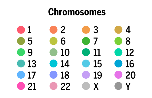
chromosomes
The lengths of the chromosomes in the latest version of the human genome assembly (hg38, December 2013) are as follows.
 1 len 248,956,422 clen   248,956,422
 2 len 242,193,529 clen   491,149,951
 3 len 198,295,559 clen   689,445,510
 4 len 190,214,555 clen   879,660,065
 5 len 181,538,259 clen 1,061,198,324
 6 len 170,805,979 clen 1,232,004,303
 7 len 159,345,973 clen 1,391,350,276
 8 len 145,138,636 clen 1,536,488,912
 9 len 138,394,717 clen 1,674,883,629
10 len 133,797,422 clen 1,808,681,051
11 len 135,086,622 clen 1,943,767,673
12 len 133,275,309 clen 2,077,042,982
13 len 114,364,328 clen 2,191,407,310
14 len 107,043,718 clen 2,298,451,028
15 len 101,991,189 clen 2,400,442,217
16 len  90,338,345 clen 2,490,780,562
17 len  83,257,441 clen 2,574,038,003
18 len  80,373,285 clen 2,654,411,288
19 len  58,617,616 clen 2,713,028,904
20 len  64,444,167 clen 2,777,473,071
21 len  46,709,983 clen 2,824,183,054
22 len  50,818,468 clen 2,875,001,522
 x len 156,040,895 clen 3,031,042,417
 y len  57,227,415 clen 3,088,269,832
There are other scaffold entries in the assembly file (e.g. chr M and unanchored segments) but these were omitted from the graphic. The mitochondrial chromosome is only 16,569 bp long, which corresponds to only 0.2 mm on the cover.
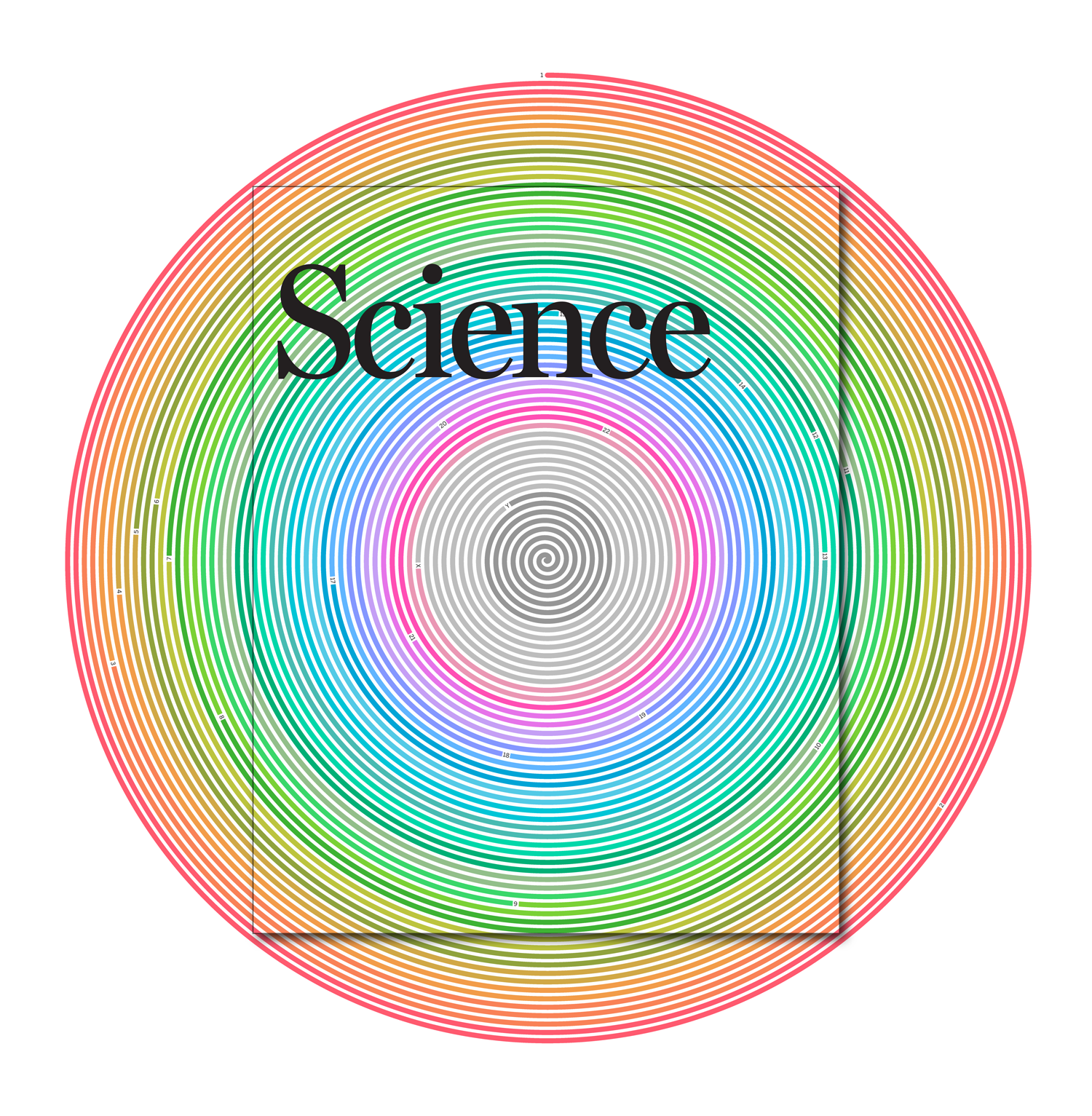
revenge of the rainbow color palette
The chromosome color palette used in the UCSC genome browser is this

One of the things the original UCSC color palette doesn't get exactly right is luminance normalization. Some colors are very bright (e.g. chr10 yellow) while others are very dark (e.g. chr14 blue). Given that bright elements (generally) command more attention than dark ones, most color palettes for ordinal or nominal variables have some kind of threshold to how much luminance (and chroma) can differ.
Below you can see the UCSC color palette normalized to luminance `L = 70, 80, 90`. While this kind of normalization satisifes some technical requirements for perceptual uniformity, these palettes lack vigor. For strict visualization you probably don't want vigor, but for artistic treatments you probably do.

A while back I looked into generating color palettes of maximally distinct colors. These palettes are formed by clustering all possible colors using perceptually uniform metric (e.g. CIE 2000 `\Delta E`) into `n` clusters. The centroid of each cluster gives the color and, as a set, these centroids are reasonably distributed through color space (e.g. Lab) in such a way that the `\Delta E` between any color and its closest neighbour is roughly the same.
I knew that I was going to make chromosomes X and Y grey, so all I needed were 22 maximally distinct colors for chromosomes 1 – 22. To select these colors, I took all colors in the LCH range `L = [60,80]`, `C = [20,100]` and `H = [0,359]` (all hues) and sampled them every `\Delta L = 5`, `\Delta C = \Delta H = 1`. This yielded 24,928 colors.
picking colors lum 60 ncolors 0
picking colors lum 65 ncolors 5715
picking colors lum 70 ncolors 10975
picking colors lum 75 ncolors 15925
picking colors lum 80 ncolors 20602
initial colors 24928
As I was building the list, any colors within `\Delta E_\textrm{00} < 2` a color already in the list were rejected (to speed up the calculations). This reduced the number of colors to cluster from 24,928 to 6,240.
removing nearby colors within dE00 2
filtering colors 0 nfiltered 0
filtering colors 1000 nfiltered 5159
filtering colors 2000 nfiltered 8600
filtering colors 3000 nfiltered 11024
filtering colors 4000 nfiltered 12728
filtering colors 5000 nfiltered 13947
filtering colors 6000 nfiltered 14958
filtering colors 7000 nfiltered 15673
filtering colors 8000 nfiltered 16261
filtering colors 9000 nfiltered 16698
filtering colors 10000 nfiltered 17084
filtering colors 11000 nfiltered 17442
filtering colors 12000 nfiltered 17697
filtering colors 13000 nfiltered 17891
filtering colors 14000 nfiltered 18037
filtering colors 15000 nfiltered 18147
filtering colors 16000 nfiltered 18269
filtering colors 17000 nfiltered 18346
filtering colors 18000 nfiltered 18428
filtering colors 19000 nfiltered 18483
filtering colors 20000 nfiltered 18541
filtering colors 21000 nfiltered 18584
filtering colors 22000 nfiltered 18624
filtering colors 23000 nfiltered 18657
filtering colors 24000 nfiltered 18679
got 6240 colors
Clustering was done using `k`-means with `\Delta E_\textrm{94}` as the distance metric. It's much faster than `\Delta E_\textrm{00}` and only subtly different.

This color cluster centroids are
#        R   G   B   L   C   H    nearest & distance
i    0 235 161 135  72  34  46 j  1 dE00 11.64
i    1 255 126  70  68  72  48 j  0 dE00 11.64
i    2 246 158  67  72  64  66 j  3 dE00 12.04
i    3 216 173  84  73  51  83 j  2 dE00 12.04
i    4 187 186  58  73  63 103 j  5 dE00 10.88
i    5 169 184 118  72  35 116 j  4 dE00 10.88
i    6 145 205  64  76  73 123 j  7 dE00  9.54
i    7  88 183  68  66  69 135 j  8 dE00  9.06
i    8  64 214 110  76  73 146 j  7 dE00  9.06
i    9 123 193 144  72  36 151 j  8 dE00 11.02
i   10   0 208 161  73  62 171 j  9 dE00 11.90
i   11  86 195 191  72  32 194 j 12 dE00 12.86
i   12   0 206 221  71  74 201 j 11 dE00 12.86
i   13  79 189 227  72  34 235 j 11 dE00 14.52
i   14 111 176 255  71  51 277 j 15 dE00 13.47
i   15 166 166 249  70  45 295 j 16 dE00 12.71
i   16 210 140 255  70  73 313 j 15 dE00 12.71
i   17 252 123 223  69  67 335 j 18 dE00 11.58
i   18 212 163 219  73  34 323 j 17 dE00 11.58
i   19 243 152 176  72  37   2 j 20 dE00 12.56
i   20 255  83 166  66  78   0 j 17 dE00 12.40
i   21 255 110 117  67  67  24 j 19 dE00 14.34
Each color is indentified by index `i`. Its closest neighbour (in terms of `\Delta E`) is color `j` and the distance between them is `\Delta E_{\textrm{00}}`. You can see that this distance to the nearest neighbour is reasonably constant(ish) (average difference is 12.3).
Note that there are two color pairs with very similar hue (`i = 0,1` and `i = 19,20`).
There are lots of greenish colors — this reflects the fact that green occupies a relatively large part of the color space.
other palette options
It's worth exploring a few different clustering scenarios, which differ by how colors to be clustered are sampled across luminance and chroma. For example, option "I" clusters 2,544 colors sampled from ranges `L = [60,80]` and `C = [80,100]` (very saturated). If we restrict color sampling to a single luminance and chroma, we get something like option "O", which clusters 104 colors with `L = 60` and `C = 80`.
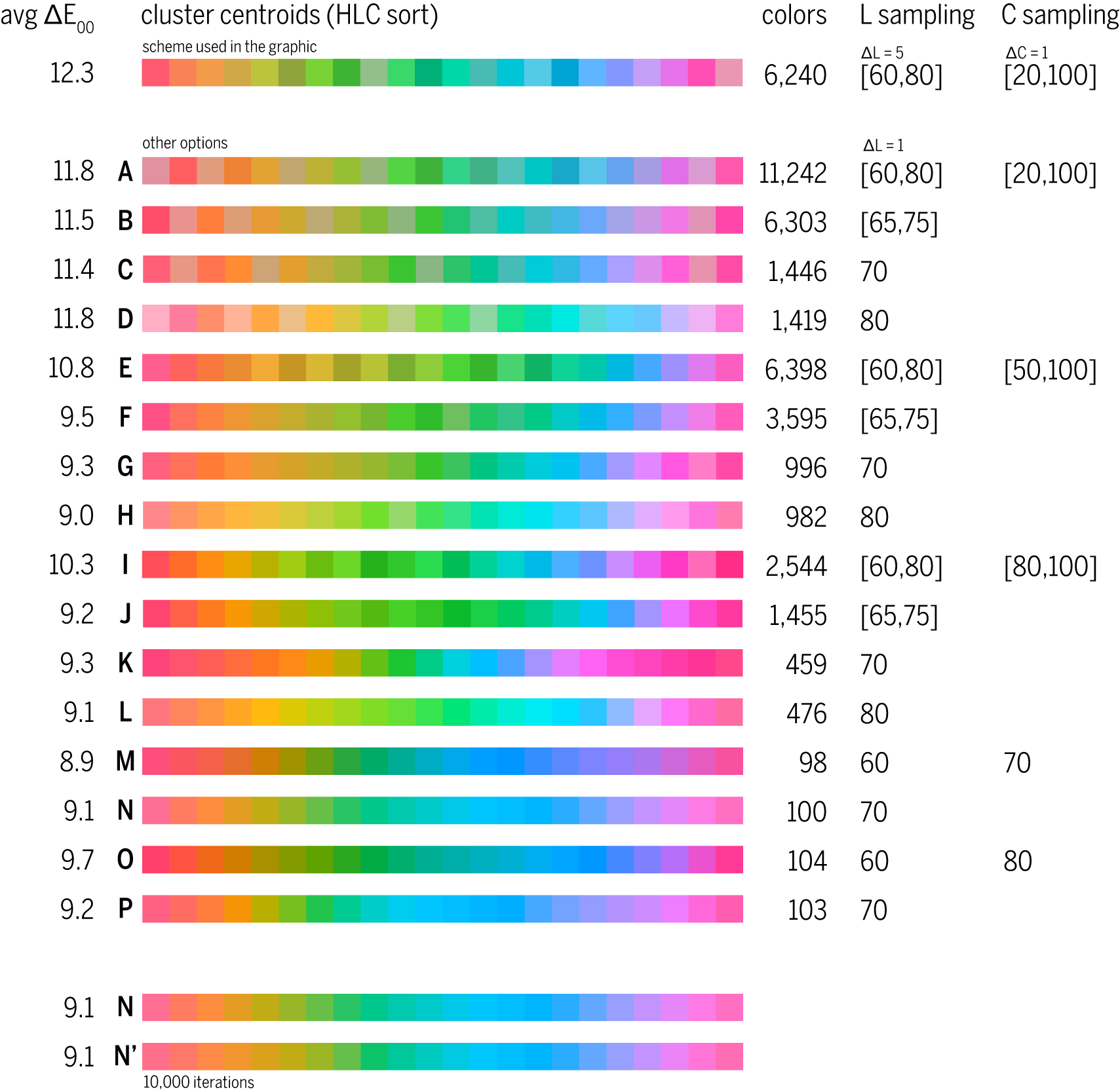
If we want 22 colors that then it's necessary to sample from a variety of luminance and chroma values. Otherwise, colors vary only by hue and some are difficult to discern. For example, in option "N" which samples from fixed `L = C = 70`, the clustering gives
i    0 255 124  98  70  69  37 j 1 dE00 14.25
i    1 255 141  63  70  69  57 j 2 dE00 14.19
i    2 228 157  35  70  69  75 j 1 dE00 14.19
i    3 193 172  21  70  69  95 j 4 dE00 13.21
i    4 151 183  41  70  69 114 j 5 dE00 10.02
i    5 104 191  72  70  69 133 j 6 dE00  7.50
i    6  40 196 101  70  69 148 j 5 dE00  7.50
i    7   0 199 140  70  69 166 j 8 dE00  8.93
i    8   0 201 174  70  69 182 j 9 dE00  7.97
i    9   0 201 202  70  69 195 j 8 dE00  7.97
i   10   0 200 233  70  69 210 j 11 dE00  6.85
i   11   0 198 255  70  69 224 j 10 dE00  6.85
i   12   0 190 255  70  69 249 j 13 dE00  9.47
i   13   0 181 255  70  69 266 j 14 dE00  8.43
i   14  43 173 255  70  69 278 j 15 dE00  5.53
i   15  99 168 255  70  69 285 j 14 dE00  5.53
i   16 152 159 255  70  69 296 j 15 dE00  9.75
i   17 195 147 255  70  69 308 j 18 dE00  8.99
i   18 230 134 251  70  69 322 j 19 dE00  6.60
i   19 254 122 228  70  69 335 j 18 dE00  6.60
i   20 255 112 195  70  69 351 j 19 dE00  7.76
i   21 255 110 148  70  69  12 j 20 dE00 11.42
If I increase the number of k-means iterations to 10,000 (from a modest 10) (see options N and N' in the figure above), then we get a set where minimum `\Delta E` varies much less. We still have the same average `\textrm{avg} \Delta E = 9.1`.
> more colors.22.txt
i    0 255 121 106  70  69  32 j 1 dE00 10.86
i    1 255 111 140  70  69  15 j 2 dE00 10.28
i    2 255 110 181  70  69 357 j 3 dE00  7.98
i    3 255 118 216  70  69 340 j 2 dE00  7.98
i    4 235 132 247  70  69 324 j 3 dE00  8.37
i    5 195 147 255  70  69 308 j 4 dE00 10.07
i    6 151 159 255  70  69 296 j 7 dE00  9.60
i    7  99 168 255  70  69 285 j 8 dE00  5.53
i    8  43 173 255  70  69 278 j 7 dE00  5.53
i    9   0 181 255  70  69 266 j 8 dE00  8.43
i   10   0 190 255  70  69 249 j 9 dE00  9.47
i   11   0 199 253  70  69 222 j 12 dE00  7.87
i   12   0 201 225  70  69 206 j 11 dE00  7.87
i   13   0 201 192  70  69 191 j 12 dE00  9.32
i   14   0 200 154  70  69 173 j 13 dE00 10.41
i   15  14 196 106  70  69 150 j 16 dE00  8.17
i   16 101 191  74  70  69 134 j 15 dE00  8.17
i   17 157 182  38  70  69 112 j 18 dE00 11.78
i   18 193 172  21  70  69  95 j 19 dE00 10.42
i   19 219 161  29  70  69  80 j 18 dE00 10.42
i   20 242 150  47  70  69  66 j 19 dE00 10.59
i   21 255 137  71  70  69  52 j 20 dE00 10.84
If we're only clustering 102 colors, then 10,000 iterations is practical.
If only one component is varying, clustering isn't very efficient. A better way to select colors in this case would be to step along the component and select adjacent colors based on a fixed `\Delta E`.
cytogenetic bands
Cytogenetic bands are chromosome landmarks obtained by Giemsa staining.
For these colors, I sampled from the grey Brewer palette. Stalks are variable regions in the five acrocentric chromosomes that connect the small arm to the chromosome.
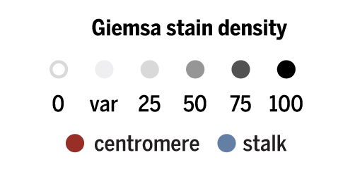
The bands were composited on top of chromosomes at 30% opacity.
The the bands and chromosomes were further muted on the cover with a faint white overlay and two gradients were added to provide visibility to text.
genes
The genes in the graphic are taken from the OMIM database, which tracks genes associated with Mendelian disorders.
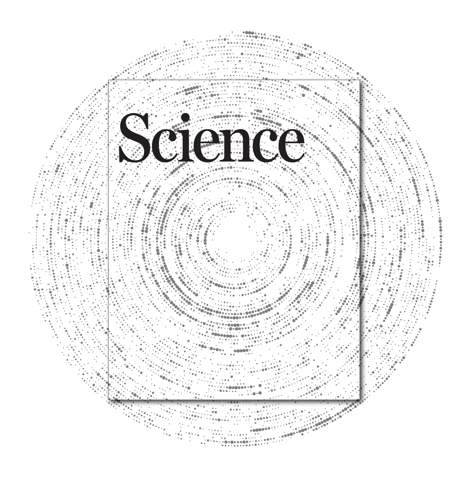
In the 2021-08-20 version of the database, there were 17,638 entries. The genomic position of each entry was taken as the midpoint between start and end position and the number of entry in each 250 kb region was tallied.
There were 6,973 regions that had non-zero counts of OMIM entries. The exact count of regions with a given number of entries is below. For example, there were 24 regions with 10 entries.
omim all 6973
omim 1 3097 size 1.0083
omim 2 1607 size 1.49850609149058
omim 3 846 size 1.88934938415614
omim 4 515 size 2.22703610655001
omim 5 290 size 2.53000291563677
omim 6 178 size 2.80789602411182
omim 7 136 size 3.06653415956866
omim 8 84 size 3.30975619521437
omim 9 68 size 3.54025696262142
omim 10 24 size 3.76001664243838
omim 11 42 size 3.97054229000266
omim 12 32 size 4.17301328612888
omim 13 12 size 4.36837373638714
omim 14 8 size 4.55739374975462
omim 15 9 size 4.74071154475013
omim 16 7 size 4.91886325486207
omim 17 6 size 5.09230456765918
omim 18 2 size 5.26142678164251
omim 19 1 size 5.4265689495722
omim 21 1 size 5.74606211035883
omim 22 1 size 5.90090430238019
omim 23 2 size 6.05275922451503
omim 24 1 size 6.2018107994994
omim 25 1 size 6.34822448986466
omim 26 2 size 6.4921498104568
omim 27 1 size 6.63372241603022
The last value in the list above is the radius of the circle used to encode the number of events in a region. The Flannery compensation was used in this encoding $$ r = 1.0083 r_0 \left( c/c_\textrm{min} \right)^{0.5716} $$
where `r_0` is the minimum radius, `c` is the count and `c_\textrm{min}` is the minimum count.
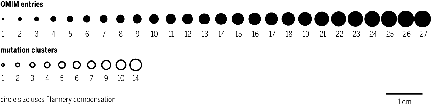
The same scheme was used for the mutation cluster circles.
mutation clusters
Mutation clusters were taken from Pan-cancer analysis of advanced patient tumors reveals interactions between therapy and genomic landscapes. (Pleasance E et al. (2020) Nature Cancer 1:452–468).

There were 2,596 clusters and their bin counts and circle sizes were as follows
cluster all 1823
cluster 1 1323 size 1.0083
cluster 2 343 size 1.49850609149058
cluster 3 96 size 1.88934938415614
cluster 4 38 size 2.22703610655001
cluster 5 10 size 2.53000291563677
cluster 6 6 size 2.80789602411182
cluster 7 4 size 3.06653415956866
cluster 9 1 size 3.54025696262142
cluster 10 1 size 3.76001664243838
cluster 14 1 size 4.55739374975462
Propensity score matching
I don’t have good luck in the match points. —Rafael Nadal, Spanish tennis player
In many experimental designs, we need to keep in mind the possibility of confounding variables, which may give rise to bias in the estimate of the treatment effect.
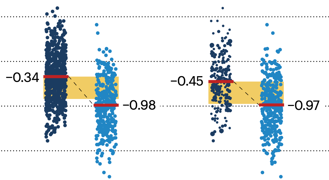
If the control and experimental groups aren't matched (or, roughly, similar enough), this bias can arise.
Sometimes this can be dealt with by randomizing, which on average can balance this effect out. When randomization is not possible, propensity score matching is an excellent strategy to match control and experimental groups.
Kurz, C.F., Krzywinski, M. & Altman, N. (2024) Points of significance: Propensity score matching. Nat. Methods 21:1770–1772.
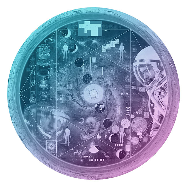
Nasa to send our human genome discs to the Moon
We'd like to say a ‘cosmic hello’: mathematics, culture, palaeontology, art and science, and ... human genomes.


Comparing classifier performance with baselines
All animals are equal, but some animals are more equal than others. —George Orwell
This month, we will illustrate the importance of establishing a baseline performance level.
Baselines are typically generated independently for each dataset using very simple models. Their role is to set the minimum level of acceptable performance and help with comparing relative improvements in performance of other models.
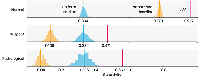
Unfortunately, baselines are often overlooked and, in the presence of a class imbalance, must be established with care.
Megahed, F.M, Chen, Y-J., Jones-Farmer, A., Rigdon, S.E., Krzywinski, M. & Altman, N. (2024) Points of significance: Comparing classifier performance with baselines. Nat. Methods 21:546–548.
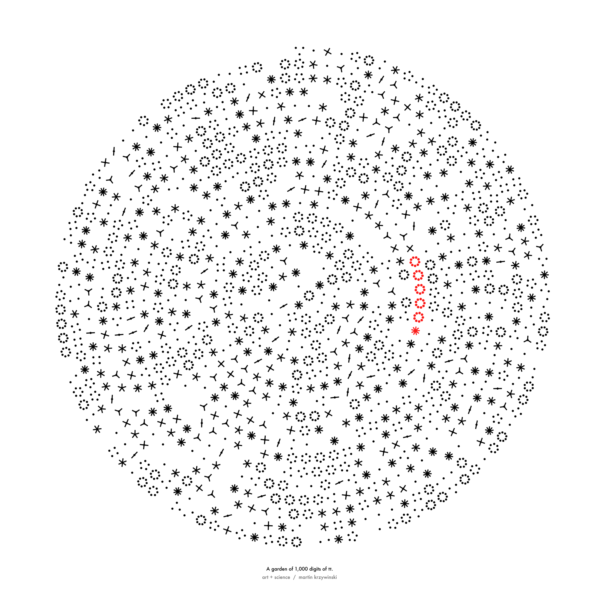
Happy 2024 π Day—
sunflowers ho!
Celebrate π Day (March 14th) and dig into the digit garden. Let's grow something.
How Analyzing Cosmic Nothing Might Explain Everything
Huge empty areas of the universe called voids could help solve the greatest mysteries in the cosmos.
My graphic accompanying How Analyzing Cosmic Nothing Might Explain Everything in the January 2024 issue of Scientific American depicts the entire Universe in a two-page spread — full of nothing.
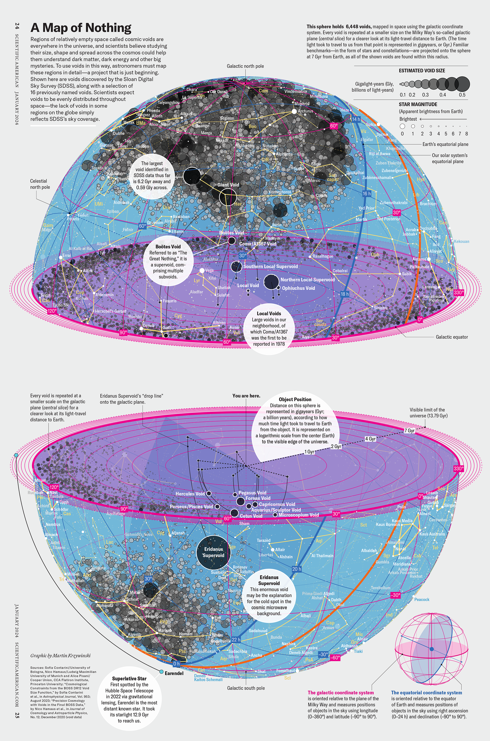
The graphic uses the latest data from SDSS 12 and is an update to my Superclusters and Voids poster.
Michael Lemonick (editor) explains on the graphic:
“Regions of relatively empty space called cosmic voids are everywhere in the universe, and scientists believe studying their size, shape and spread across the cosmos could help them understand dark matter, dark energy and other big mysteries.
To use voids in this way, astronomers must map these regions in detail—a project that is just beginning.
Shown here are voids discovered by the Sloan Digital Sky Survey (SDSS), along with a selection of 16 previously named voids. Scientists expect voids to be evenly distributed throughout space—the lack of voids in some regions on the globe simply reflects SDSS’s sky coverage.”
voids
Sofia Contarini, Alice Pisani, Nico Hamaus, Federico Marulli Lauro Moscardini & Marco Baldi (2023) Cosmological Constraints from the BOSS DR12 Void Size Function Astrophysical Journal 953:46.
Nico Hamaus, Alice Pisani, Jin-Ah Choi, Guilhem Lavaux, Benjamin D. Wandelt & Jochen Weller (2020) Journal of Cosmology and Astroparticle Physics 2020:023.
Sloan Digital Sky Survey Data Release 12
Alan MacRobert (Sky & Telescope), Paulina Rowicka/Martin Krzywinski (revisions & Microscopium)
Hoffleit & Warren Jr. (1991) The Bright Star Catalog, 5th Revised Edition (Preliminary Version).
H0 = 67.4 km/(Mpc·s), Ωm = 0.315, Ωv = 0.685. Planck collaboration Planck 2018 results. VI. Cosmological parameters (2018).
constellation figures
stars
cosmology