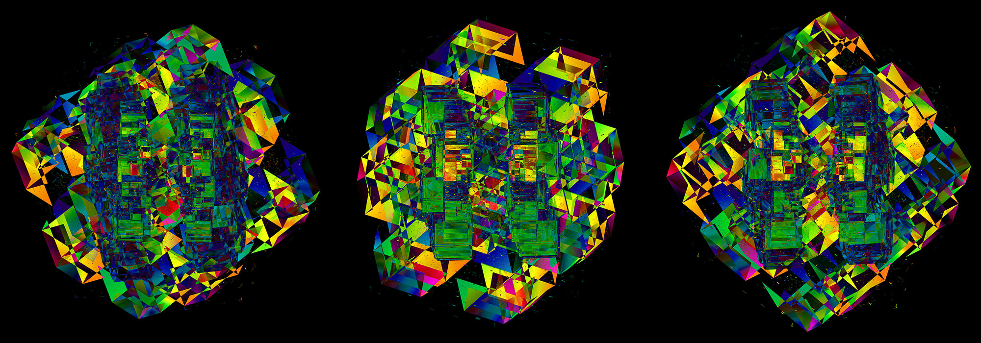
Max Cooper's Ascent — Making of the Music video
Enter the 5th dimension
contents
The scene takes place on a 5-dimensional stage, which is projected onto two dimensions (without perspective). Over time, cubes appear on the stage. Throughout the video, both the camera and each cube can rotate independently.
For some cubes, area maps of the digits of `\pi` or its approximations (e.g. 22/7) are projected onto some of the faces of the cube.
The video was created with a custom animation system that I wrote specifically for Ascent.
The animation is structured around a series of keyframes. Each keyframe (there are about 170 keyframes) is defined using a custom scripting language with which I can add elements to the scene, apply a rotation, zoom and scale, project area maps, and so on.
The keyframes were created manually and the motion was designed to match the dynamics and movement of the music. There is no automated synchronization.
For example, the first 8 seconds of the video is created from these keyframe definitions.
# parameter definitions
...
param = fs 24
# angle in units of 2π (–17.6 deg)
param = astepa2 d-0.048978
...
# add a cube with size 0 and edge fade 1
frame = 1.a; cube_add(c0,0,1)
# rotate the scene in yw plane by 'astepa2' amount (defined elsewhere)
frame = 1.a0; a yw astepa2
# previous keyframe parameters will be interpolated over
# 2fs = 48 frames (2 seconds at 24 fps) to values of the next keyframe
# i.e. cube c0 edge fade in xy plane will linearly decrease from 1 to 0
frame = 1.a1; n 2fs; c c0 f [xy] 0
# cube c0 x size grows to 0.05
frame = 1.a2; n 2fs; c c0 s [x]  0.05
# cube c0 x size grows to 0.10
frame = 1.a3; n 2fs; c c0 s [x]  0.10
# cube c0 x size grows to 0.15
frame = 1.a4; n 2fs; c c0 s [x]  0.15
...
Here are the first four keyframes — there are 2fs = 48 interpolated frames between each of these keyframes.

c c0 f [xy] 0

c c0 f [xy] 0
c c0 s [x] 0.05
c c0 s [x] 0.05
c c0 s [x] 0.10

c c0 s [x] 0.10
c c0 s [x] 0.15
For all the keyframes, see the keyframe section.
The 5-cube (`n=5`) has `2^5=32` vertices (0-cubes, corners), `2^4 \times 5 = 80` edges (1-cubes, lines), `2^3 \times 10 = 80` faces (2-cubes, squares), `2^2 \times 10 = 40` cubic cells (3-cubes) and `2^1 \times 5 = 10` tesseract cells (4-cubes).
In general, the number of `m`-cubes in an `n`-cube is $$E_{m,n} = 2^{n-m} \binom{n}m $$
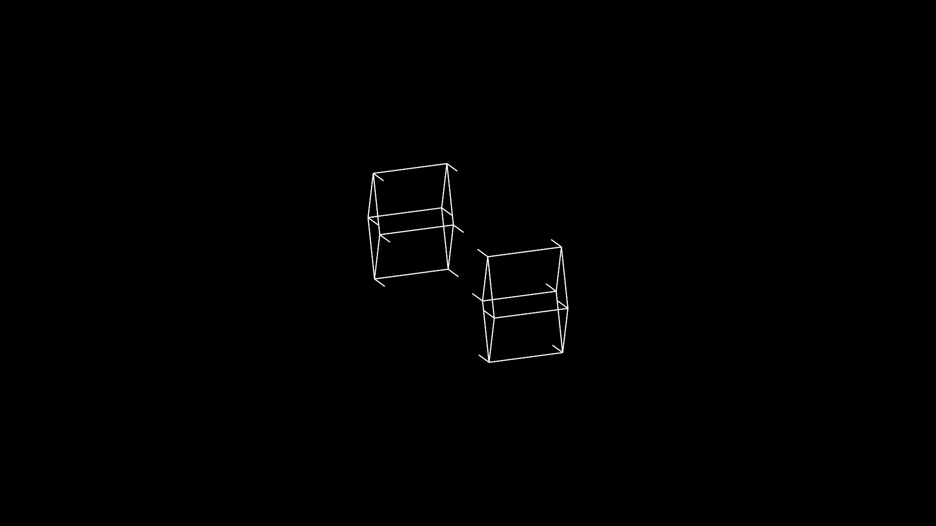
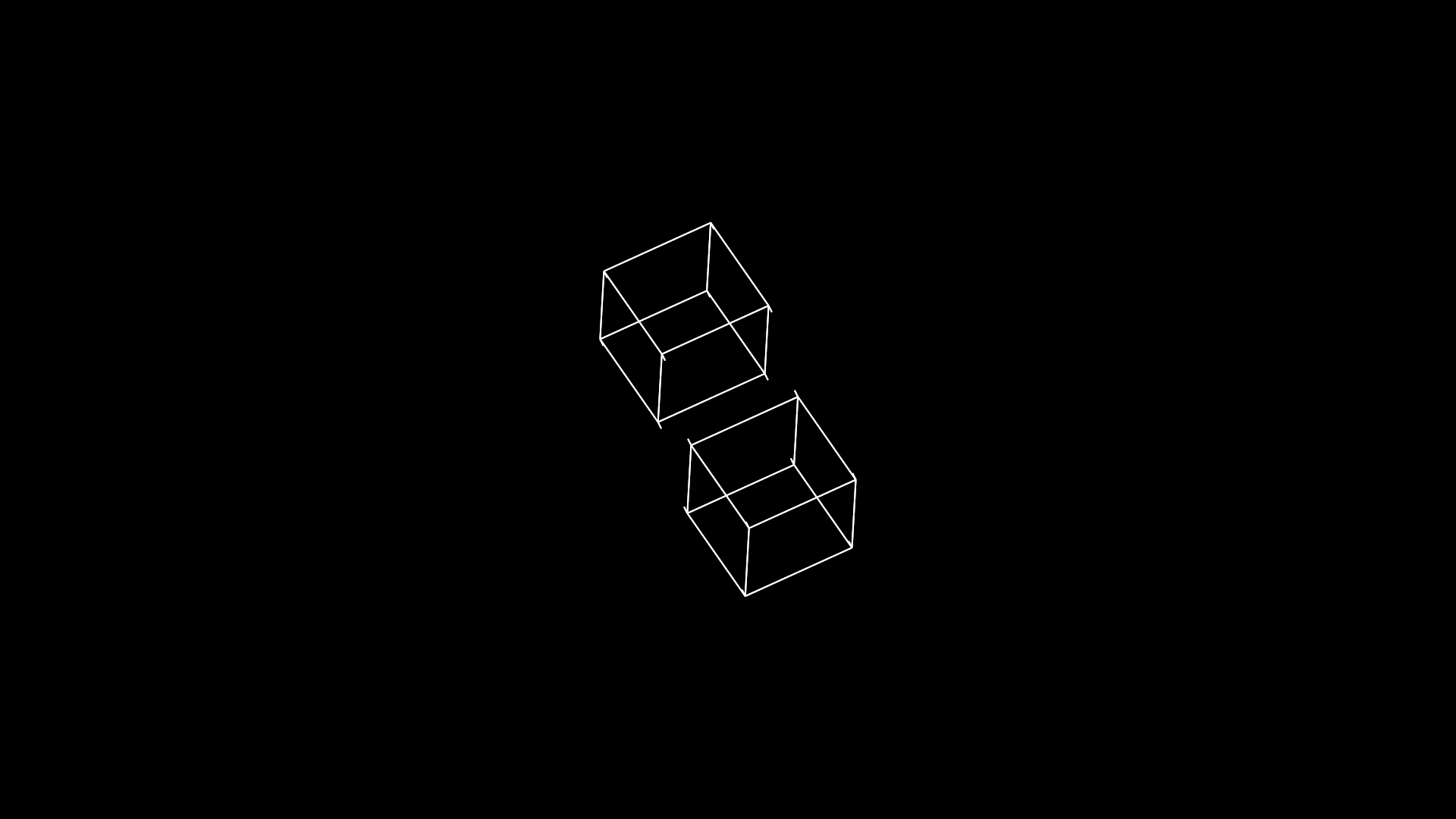
Here's a sample frame from the video — this is frame 830/8520.
It shows a pair of three dimensional cubes, each with lines growing from their vertex towards the other cube.
But what you're actually seeing is a single 5 dimensional cube, but with some dimensions collapsed and edges along other dimensions not fully drawn.
a xw astepb4
c c0 f [w] 0.9
c c0 s [w] 0.715
c c0 s [xyz] 0.15
rots
rxy2
!ryz2
a xw astepb4
c c0 f [w] 0.8
c c0 s [w] 0.615
c c0 s [xyz] 0.15
rots
rxy2
!ryz2
The view table shows the camera zoom and angle (in degrees). In 2-dimensional space there is one direction of rotation — in the `xy` plane (axis of rotation is `z`). In 3-dimensional space, there are three directions of rotation — in the `xy`, `yz` and `xz` planes. Once we reach 5 dimensions there are 10 directions of rotation (`xy`, `yz`, `xw`, `xv`, `yz`, `yw`, `yv`, `zw, `zv, `wv`).
In this frame, 7 of these angles are non-zero. It's essentially impossible to look at these angles and be able to predict how the rotated cube will look. To explore rotations in 4-dimensional space, check out Bartosz Chechanowski's excellent article on Tesseract building and rotation.
Each cube has its own angles. In this frame, the cube's angles are all zero, meaning that the rotation in the scene is due entirely to the rotation of the camera. Once more cubes are introduced, each can rotate independently to make the animation more dynamic.
There is one 5-dimensional cube in this scene (C0) and its size, edge length and rotation is presented in another table.
The cube has 5 size values, which correspond how far the cube extends into each of the dimensions. If the size `s_d` is zero then dimension `d` is collapsed. For example, if `s_w = s_v = 0` and `s_x = s_y = s_z = 1` then we just have a regular 3-cube.
In this frame, the cube has grown quite a bit in the 4th dimension `s_w = 0.64` but not as much in the first three dimensions `s_x = s_y = s_z = 0.15`. The fifth dimension is collapsed `s_v = 0`.
The cube's edge values `e_d` indicate how much of the edge along that dimension is drawn. If `e_d = 1` then the edge spans the full distance between vertices. For fractional values, the edge will extend only partially from the corner along the distance.
In this frame, the edges in the first three dimensions are fully drawn but along `w` the edge value is `e_w = 0.18` — the middle 82% of the edge is not drawn.
The combination of size and edge values can highlight lower-dimensional components of the cube — for example, by not drawing edges along certain dimension.
a xw astepb4
c c0 f [w] 0.2
c c0 s [w] 0.215
rots
rxy2
!ryz2
a xw astepb4
c c0 f [w] 0.0
c c0 s [w] 0.150
rots
rxy2
!ryz2
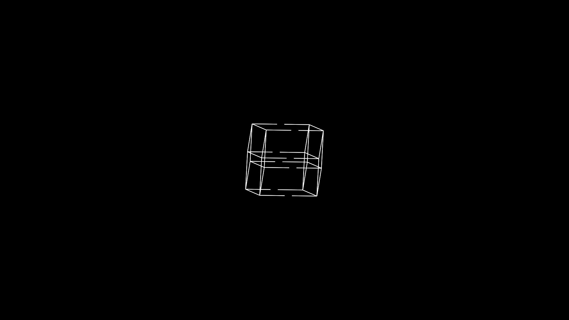
By the time we get to frame 1050, the edges along the `w` dimension are almost completely drawn (`e_w = 0.87`). But also the size of the cube along `w` has shrunk from `s_w = 0.64` to 0.19, which is very close to the size of the cube in the other dimensions (`s_{xyz} = 0.15`). This has the effect of bringing the 3-cube cells closer together.
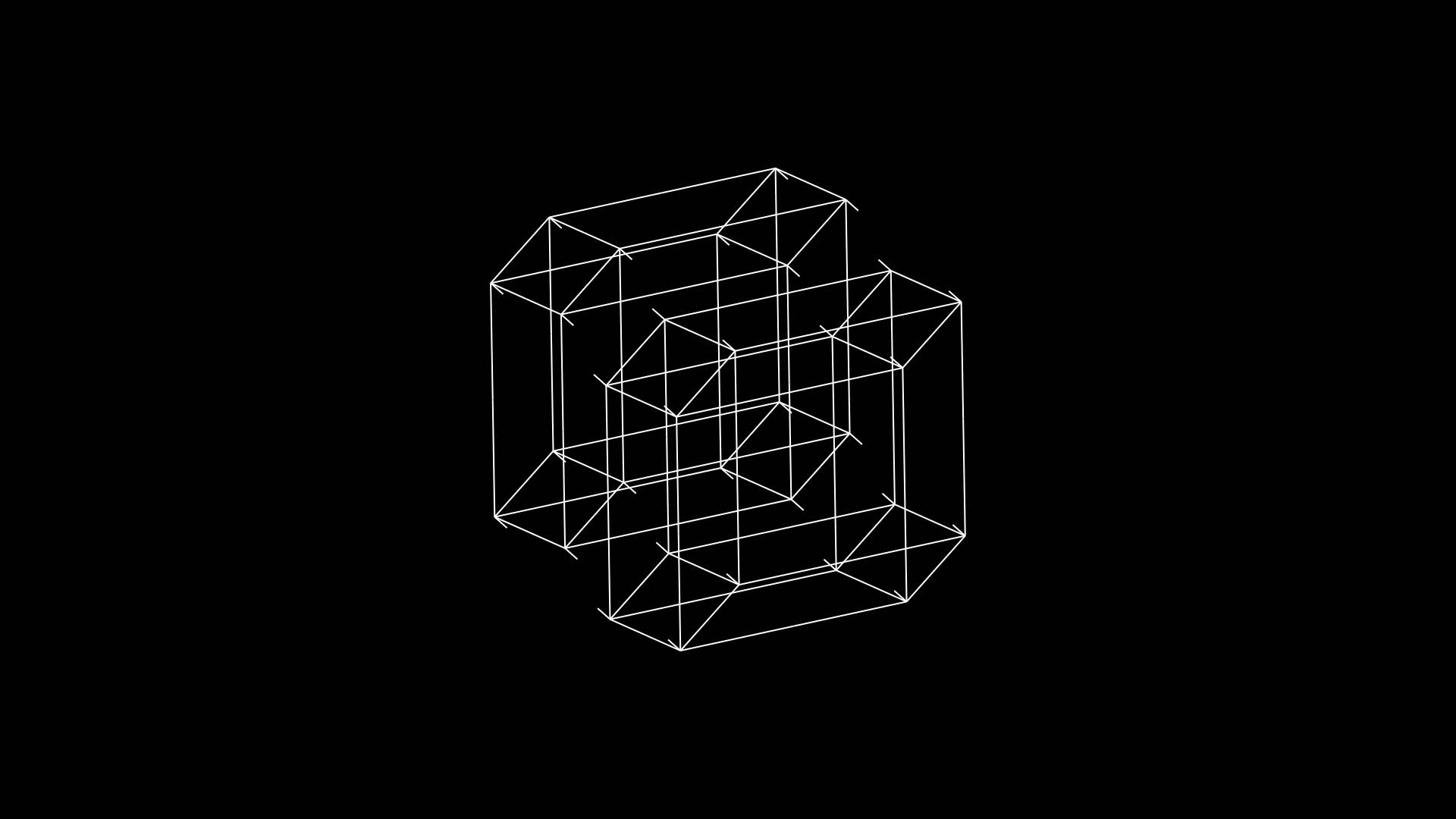
c c0 f [v] 0.80
c c0 s [xyzwv] 0.250
rots
rxy2
ryz2
c c0 f [v] 0.70
c c0 s [xyzwv] 0.275
rots
rxy2
ryz2
Shortly after, the cube's `v` dimension has grown (now the size along all dimensions is the same, `s_{xyzwv} = 0.25`) and edges are starting to form along the `v` dimension (`e_v` = 0.21).
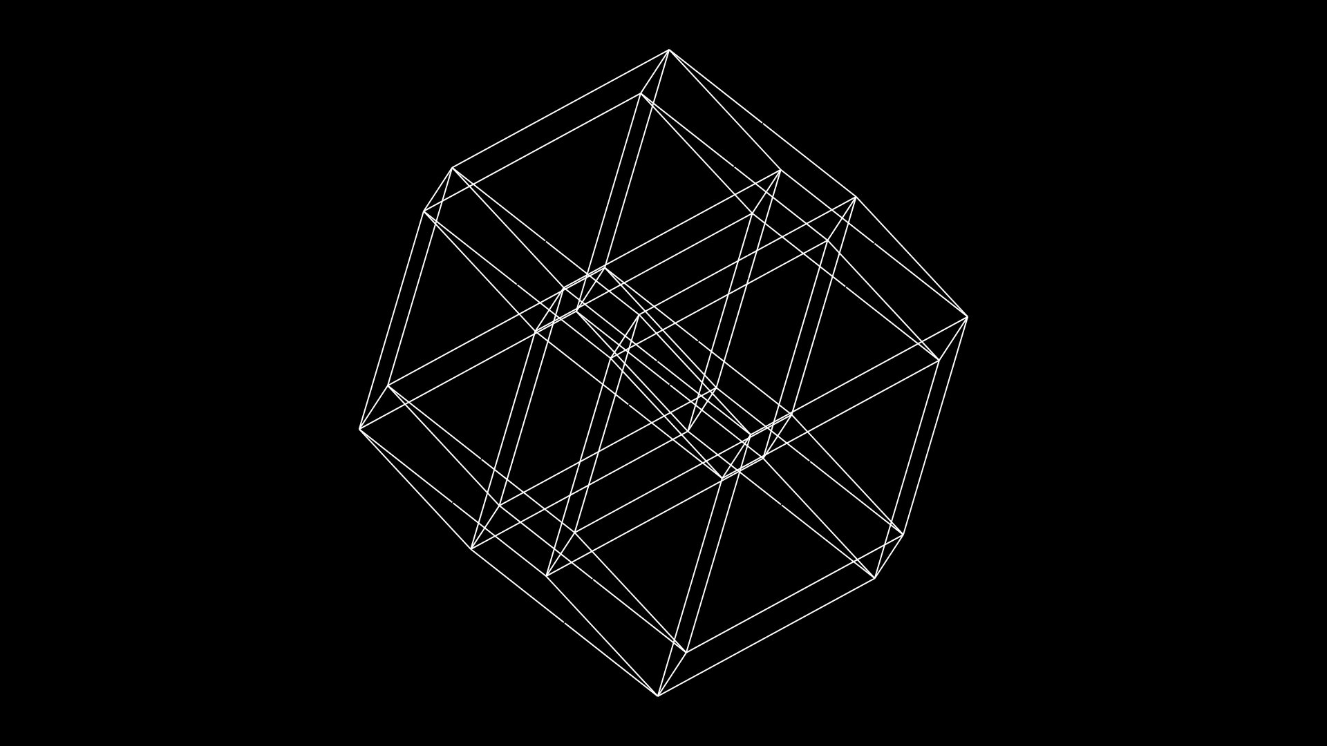
c c0 f [v] 0.10
rots
rxy2
ryz2
c c0 f [v] 0.00
rots
rxy2
ryz2
And, finally at frame 1726, we have our first complete (`s_{xyzwv} = e_{xyzwv} = 1`) 5-dimensional cube.
You now have everything that you need to interpret the full video. So, let's gets started on the walkthrough.
The walkthrough takes you through interesting landmarks in the video. It shows the frame, the keyframe before and after the frame (the frame is interpolated between these) and the parameters (size, edge, rotation, etc) of each object in the frame.
For a full list of keyframes, see the keyframe section.
Initially the scene is blank — we have one cube but its size in all dimensions is zero.

c c0 f [xy] 0
Slowly, the cube's size in the `x` dimension grows, now at `s_x = 0.14`. Edge values are `e_x = e_y = 1` meaning that the edge is completely drawn between vertices. The edge appears to grow because it's the cube that is growing (`s_x` is increasing).

c c0 s [x] 0.10
c c0 s [x] 0.15
The cube has grown to `s_x = 0.15` and is now growing in the `y` dimension (`s_y = 0.07`). Simultaneously, the scene is rotating in the `xy` plane. Note that there is an initial non-zero `yw` plane angle — this sets us up for an interesting point of view for when we start seeing the `w` dimension.
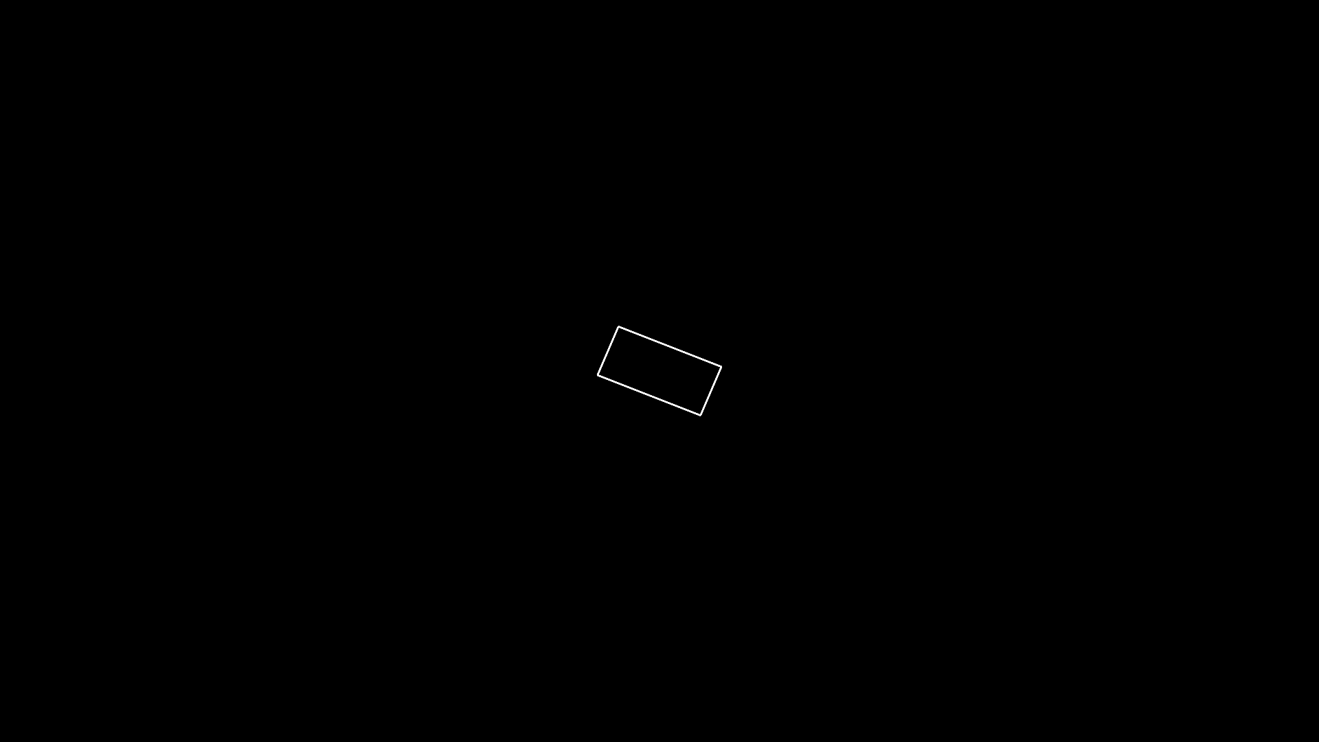
c c0 s [y] 0.05
rxy3
c c0 s [y] 0.10
rxy3
Next, the `z` diemension grows and we're finally starting to see a 3-cube form. We perceive two 2-cubes (squares) splitting up, with edges forming between them (`e_z = 0.85`). Of course, what's actually happening is that the 3-cube's `z` dimension is growing.
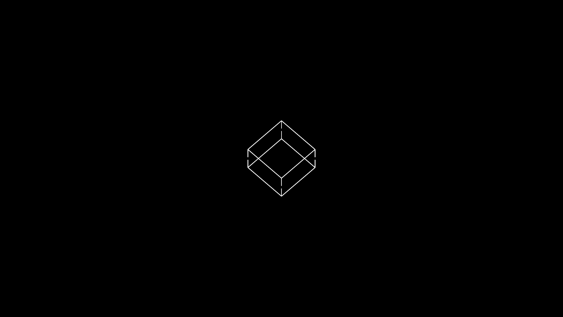
c c0 f [z] 0.20
c c0 s [xy] 0.15
c c0 s [z] 0.130
ryz6
c c0 f [z] 0.10
c c0 s [xy] 0.15
c c0 s [z] 0.140
ryz6
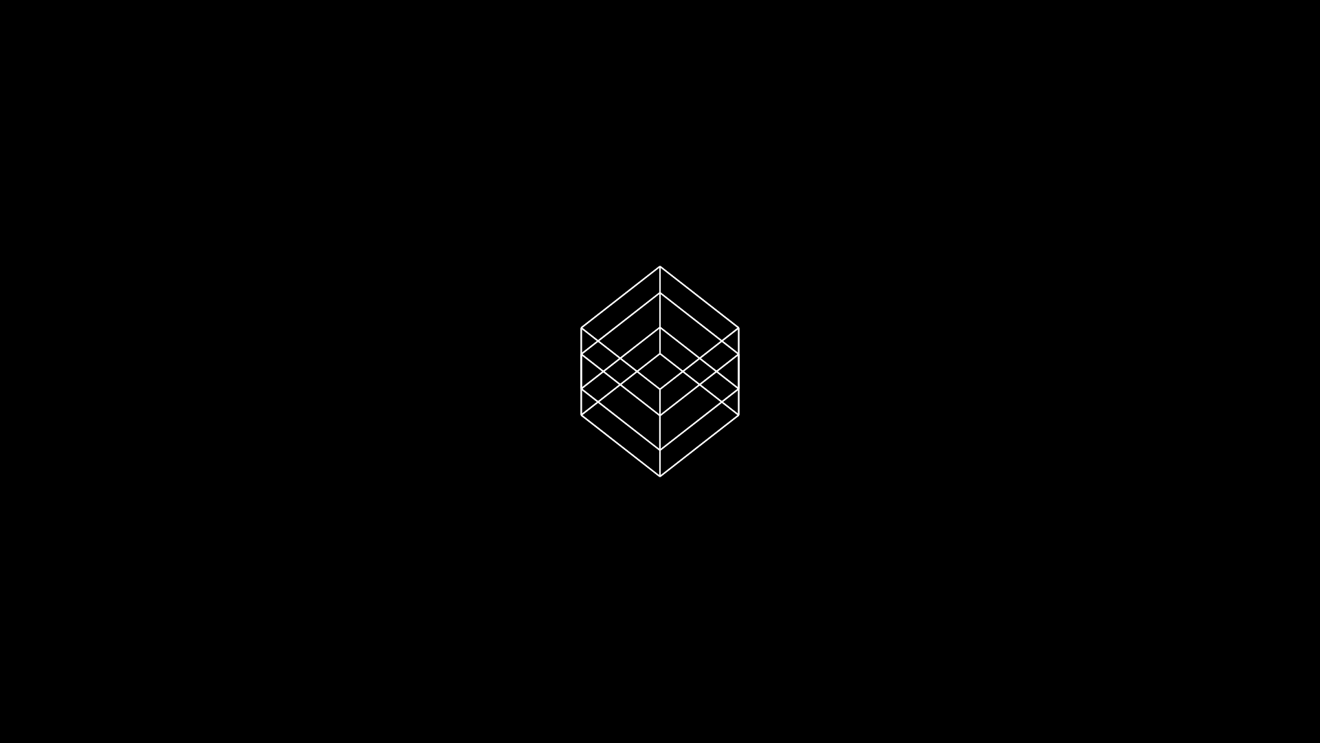
Around frame 675 is the first time we get a hint of higher dimensions. By now, the cube has grown equally in the first three dimensions (`s_{xyz} = 0.15`) and edges along these dimensions are fully formed (`e_{xyz} = 1`).
The cube now appears to be splitting into two copies because its `w` dimension is growing (`s_w = 0.12`). But, because no edges are drawn along this dimension (`e_w = 0`), the cubes don't appear to be connected in any way. Thus, we still really don't know how many dimensions this scene has — the effect is the same as if we were looking at a 3-dimensional scene in which a 3-cube splits into two.
c c0 f [z] 0.00
c c0 s [xy] 0.15
c c0 s [z] 0.150
ryz6
c c0 s [w] 0.815
c c0 s [xyz] 0.15
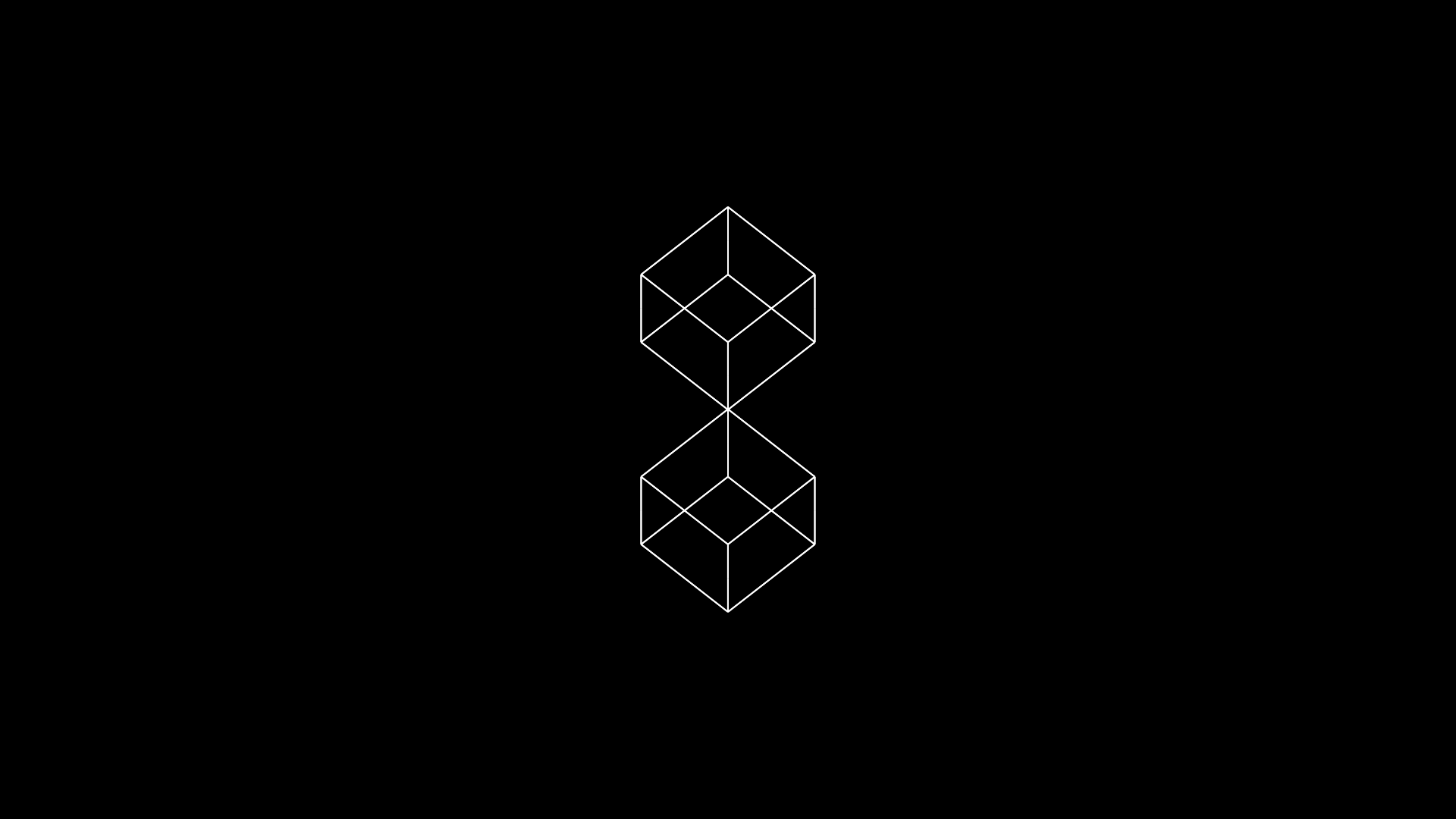
At frame 730, it looks like we have a pretty symmetric stacking of two 3-cubes but we're actually looking at a 4-cube without `w` edges and rotated in the `xy`, `yz` and `yw` planes to achieve this effect.
c c0 s [w] 0.815
c c0 s [xyz] 0.15
The scene now starts to rotate in a more complex fashion and edges along the `w` dimension begin to grow (`e_w = 0.07`) as this dimension starts to shrink (`e_w=0.74`) to the same size as (`e_{xyz} = 0.15`).
a xw astepb4
c c0 f [w] 0.9
c c0 s [w] 0.715
c c0 s [xyz] 0.15
rots
rxy2
!ryz2
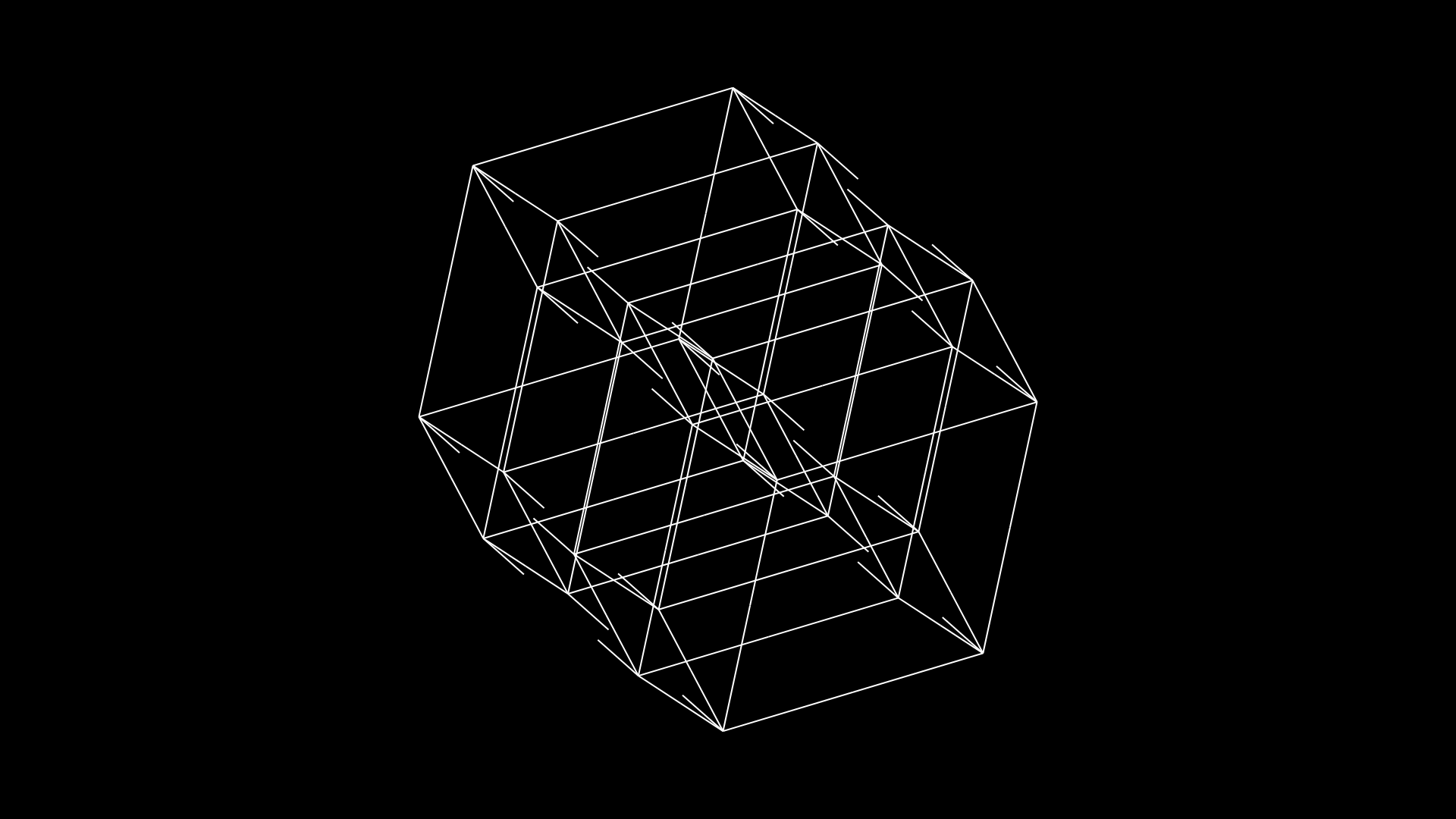
This process continues and by frame 1500, the cube's size in all dimenions is the same (`e_{xyzwv} = 0.31`) and only the edges along `v` still need to grow to completion (right now, they're about 50% extended).
c c0 f [v] 0.50
c c0 s [xyzwv] 0.300
rots
rxy2
ryz2
c c0 f [v] 0.40
c c0 s [xyzwv] 0.325
rots
rxy2
ryz2
By now, the entire scene has zoomed in a little bit — the camera zoom has increased from 1 to 1.3.
Finally, more interesting things begin to happen. Four new cubes are introduced (C1, C2, C3, C4). Initially, these have the same size in each dimension as our original cube C0, but their `e_{xyzwv} = 0`, so no edges are drawn.
Then, the edges for C1 start to grow. Initially, only in the `xy` plane (`e_{xy} = 0.36)`. These edges are drawn with a thicker line and a difference blend, so what you're seeing (in the black and white version) is something that looks like a tube growing from the vertices.
The purpose of this scene is to draw attention to the faces in the `xy` plane.
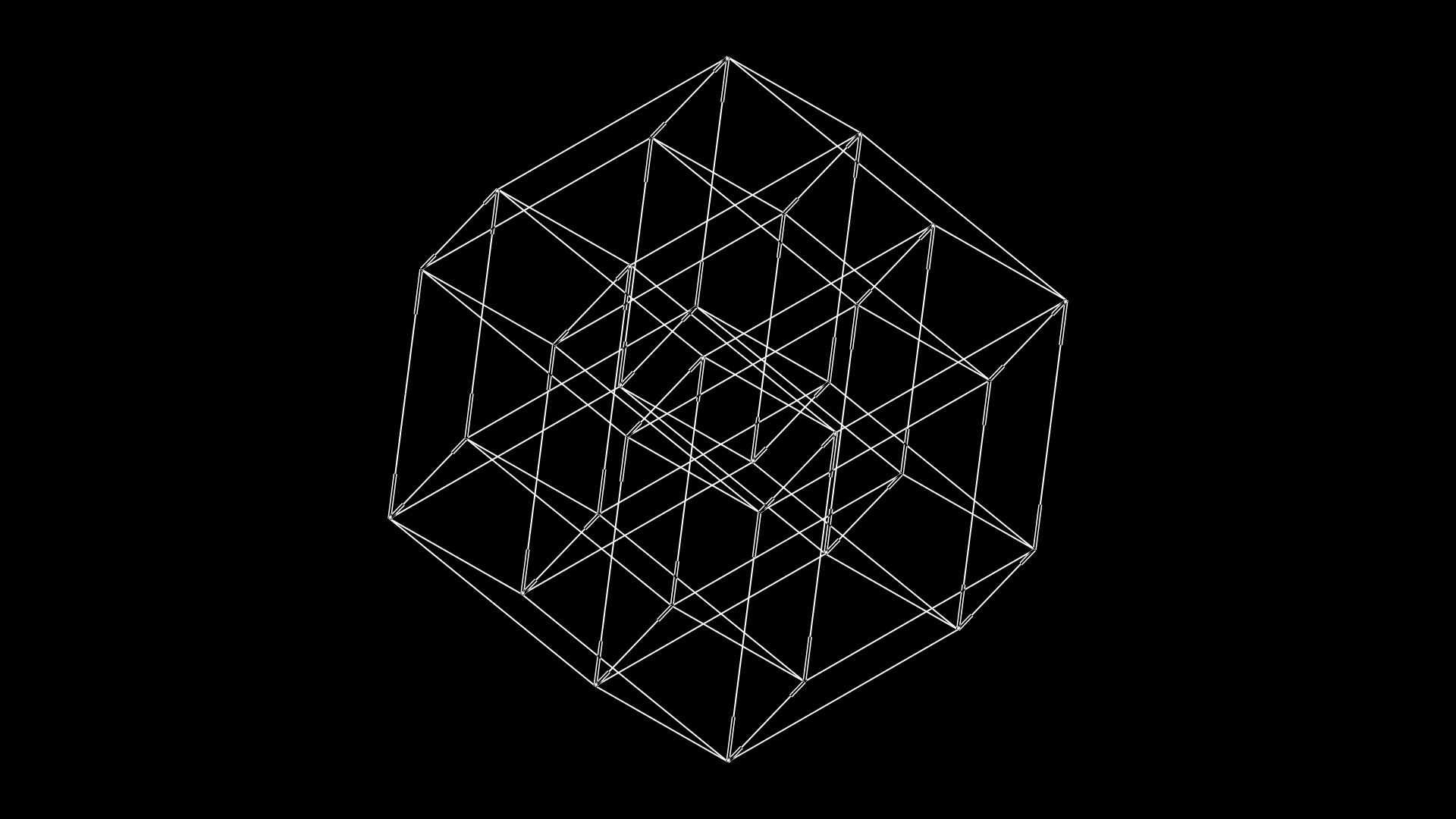
c c1 f [xy] s2f
rotthis2
c c1 f [xy] s2f
rotthis2
As the edges in C1 continue to grow, the edges in C2 in the `xz` plane start to grow (`e_{xz} = 0.46`).
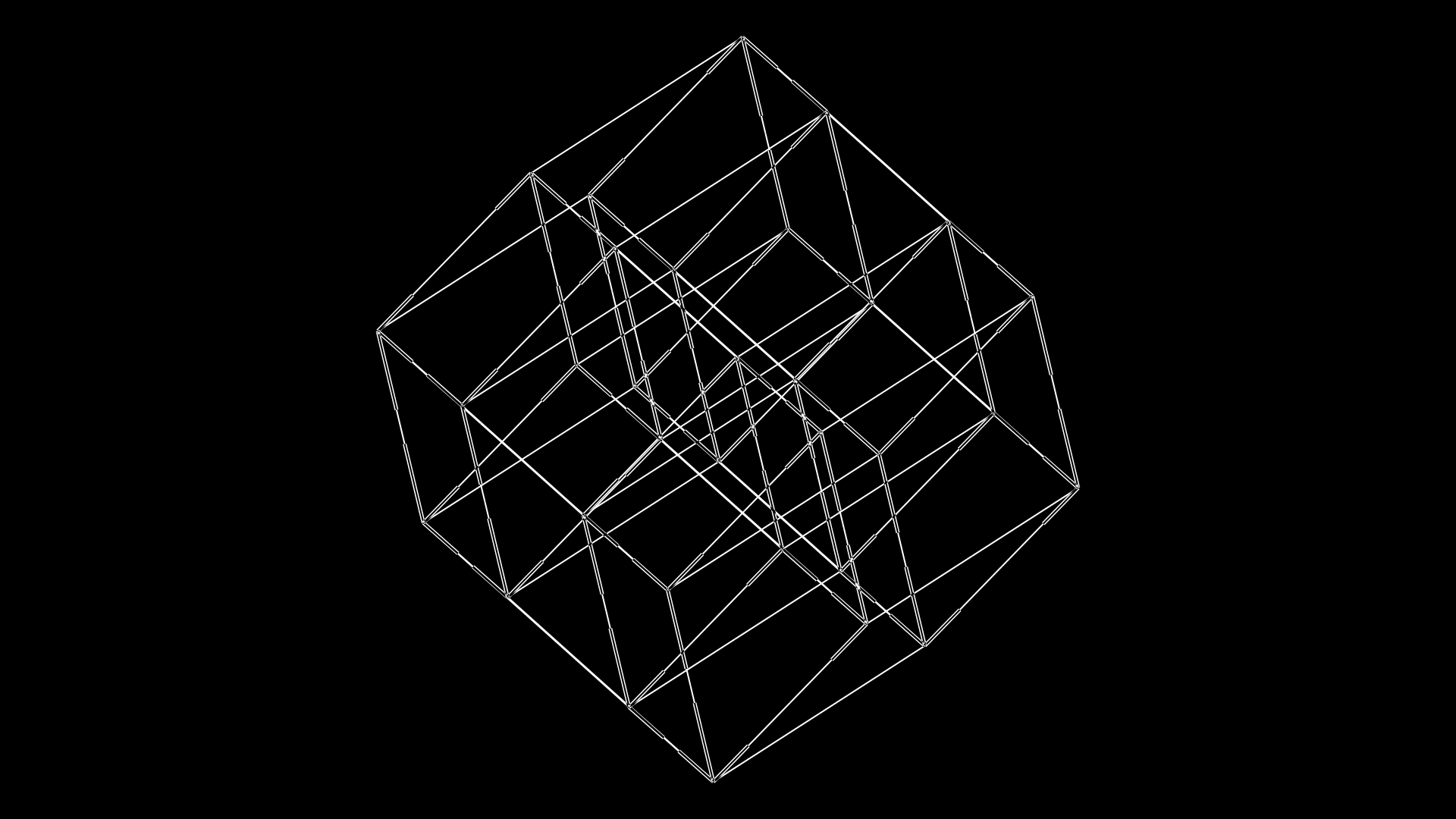
c c1 f [xy] s2f
c c2 f [xz] s2f
rotthis2
c c1 f [xy] s2f
c c2 f [xz] s2f
rotthis2
Finally, each of the C1–C4 cubes has grown its edges fully: C1 in `xy`, C2 in `xz`, C3 in `xw` and C4 in `xv`.
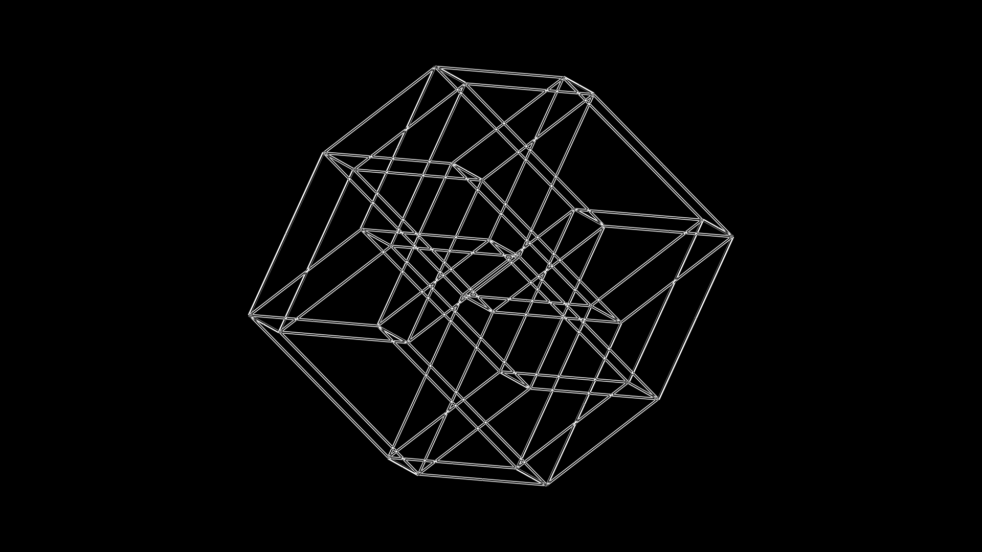
c c1 f [xy] s2f
c c2 f [xz] s2f
c c3 f [xw] s2f
c c4 f [xv] s2f
rotthis2
c c1 f [xy] 0
c c2 f [xz] 0
c c3 f [xw] 0
c c4 f [xv] 0
rotthis2
Now, something funky starts to happen. It looks like the faces from the original C0 cube are coming off. Yes they are.
This is achieved by increasing the size of the cubes C1–C4, which, if you remember, only had edges drawn within one plane (e.g. `xy`).
In this frame, cube C1 has grown from `s_{xyzwv} = 0.33` to 0.38. This is the cube that has `xy` edges (`e_x = e_y = 1`).
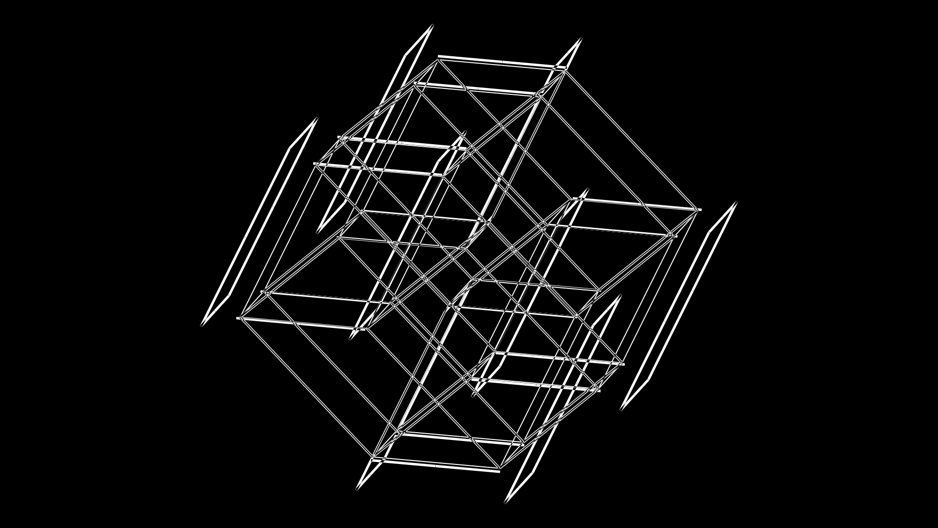
c c1 s . s3s
rotthis2
c c1 s . s3s
c c2 s . s3s
rotthis2
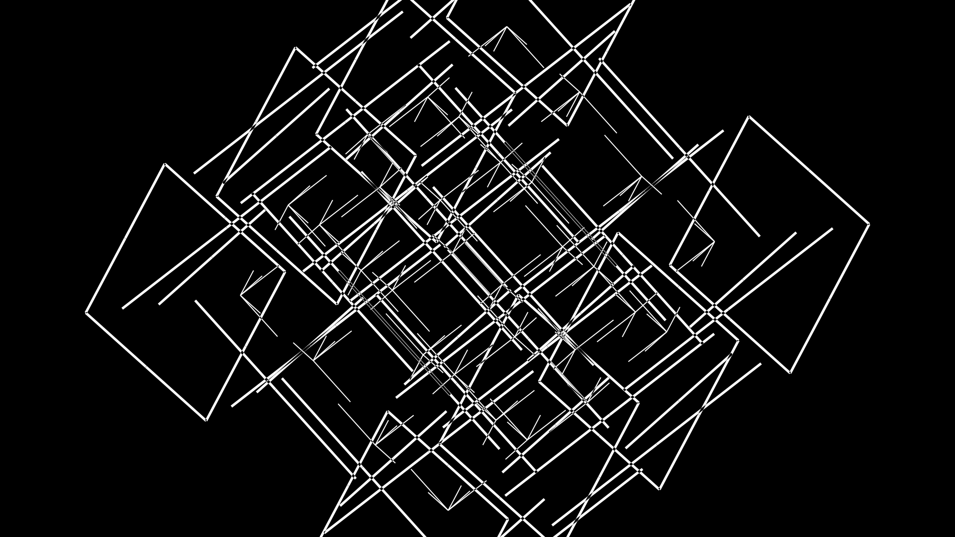
Now, quite a bit is happening but it can all be understood in terms of what you've already seen.
First, the C1–C4 cubes have grown (each to a different extent) beyond the size of C0 (which makes their faces look like they've separated). For example, C1 has `s = 0.54` whereas C4 grew less at `s = 0.39`.
The other effect is that the edges for C0 are now shrinking towards the cube's vertices — this achieved by lowering the edge size to `e = 0.55`.
c c0 f . s3f
c c[1-4] s . s3s
rotthis2
c c0 f . s3f
c c[1-4] s . s3s
rotthis2
rep 2
Ready for more? Yes you are.
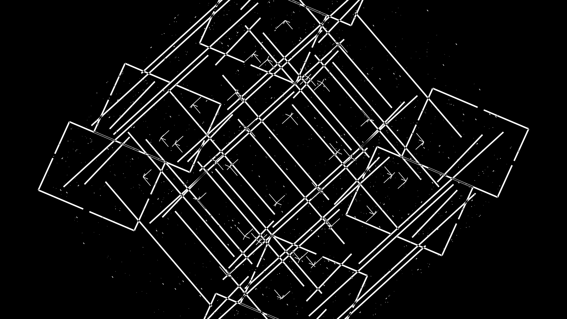
The edges of C0 have shrunk back to the cube's vertices (`e = 0.18`) so we only see 18% of the total edge length (i.e. there is a 82% gap in the middle of the edge). You'll also notice that the edges of C1 are starting to shrink (`e = 0.94`), which you can see as a small gap forming in one set of the thicker squares (e.g. first face from the right of the frame).
You're also seeing little specks form everywhere. These are the beginnings of the area maps of the digits of `\pi` (or its approximations), projected onto the faces of a cube.
c c0 f . 0.90
c c1 f [xy] s4f
c c[0-1] s . p2
map_fade(c1,.,p1)
rotthis3
size . s4u
`e` = 0.01 `z` = 1.00
`e` = 0.00 `z` = 1.00
`e` = 0.00 `z` = 1.00
`e` = 0.00 `z` = 1.00
In this frame, I've assigned maps to each of the 80 faces of cubes C1–C4. That's 300 maps. The map name reflects the digit and the levels of the map. For example, map 22a is a 2-level map of the `22/7` approximation and 22b is a 3-level version of it.
map = 10a 10/3 2
map = 10b 10/3 3
map = 10c 10/3 4
map = 22a 22/7 2
map = 22b 22/7 3
map = 22c 22/7 4
map = 179a 179/57 2
map = 179b 179/57 3
map = 179c 179/57 4
map = 245a 245/78 2
map = 245b 245/78 3
map = 245c 245/78 4
map = 355a 355/113 2
map = 355b 355/113 3
map = 355c 355/113 4
map = pia pi 2
map = pib pi 3
map = pic pi 4
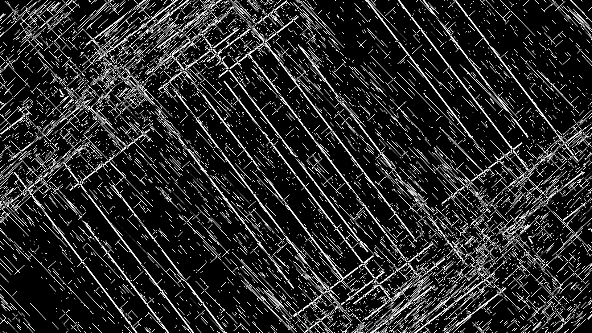
The scene keeps zooming in — now the zoom is `z = 2`. Cube C0 keeps growing `s = 0.67` and its edges continue to fade to the corners `e = 0.1`. Cubes C1–C4 keep growing and the edges of the maps on their faces are also growing. For example, cube's C1 and C2 maps have `e=0.10`.
a xv 0.10
a xw 0.90
a xz 0.16
c c2 f [xz] s4f
c c[0-2] s . p2
cube c[1-2] a [xy][yzwvu] astep-fast
map_fade(c2,.,p1)
rotthis3
size . s4u
a yv 0.15
a yw 0.03
c c3 f [xw] s4f
c c[0-3] s . p2
cube c[1-2] a [xy][yzwvu] astep-fast
map_fade(c3,.,p1)
rotthis3
size . s4u
`e` = 0.10 `z` = 1.00
`e` = 0.10 `z` = 1.00
`e` = 0.04 `z` = 1.00
`e` = 0.00 `z` = 1.00
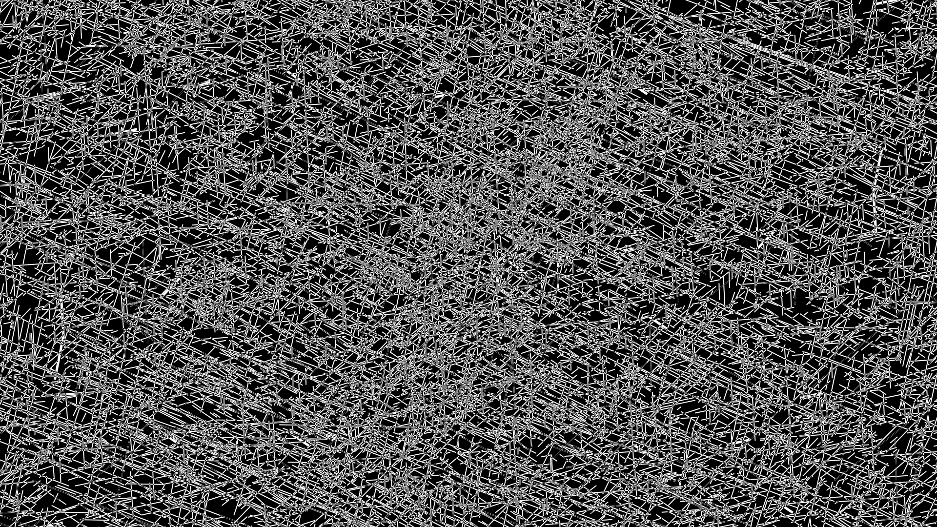
The scene continues to zoom (`z=2.59`) and the edges of all cubes have faded to corners (`e = 0.1`). The map edges are around 20% complete.
Because the scene zoomed in quite a bit now, you don't see all the corners of any given cube. Periodically, corners fly by and then quickly pass out of view.
c c4 f [xv] s4f
cube c[1-4] a [xy][yzwvu] astep-fast
map_fade(c[1-4],.,p1)
rotthis3
size . s4u
cube c[1-4] a [xy][yzwvu] astep-fast
map_fade(c[1-4],.,p1)
rotthis3
size . s4u
`e` = 0.22 `z` = 1.00
`e` = 0.22 `z` = 1.00
`e` = 0.19 `z` = 1.00
`e` = 0.16 `z` = 1.00
At this point, four more cubes are introduced into the scene: C5–C8. These cubes are different from the cubes we've already seen in that instead of shown as edges, they are shown as filled faces. Faces may be incompletely drawn (i.e. not the full face but only as square patches near their vertices.
The faces of cubes C5 and C6 are partially drawn (`e=0.16` and `e=0.09`, respectively). Faces for cubes C7 and C8 are not yet drawn (`e=0`).
c c[1-4] a [xy][yzwvu] astep-vfast
c c[5-5] f . s5cf
map_fade(c[1-4],.,s5f)
rotthis3
c c[1-5] a [xy][yzwvu] astep-vfast
c c[5-6] f . s5cf
map_fade(c[1-4],.,s5f)
rotthis3
rep 5
`e` = 0.20 `z` = 1.00
`e` = 0.20 `z` = 1.00
`e` = 0.17 `z` = 1.00
`e` = 0.14 `z` = 1.00
By now, the faces for each cube C5–C8 are being drawn (`e>0`). From this angle, the corners of these cubes are at the periphery of the viewport. At the same time, the projected area maps on cubes C1–C4 start to fade away (maps' `e` is decreasing).
Notice that each of the cubes C1–C8 has its own rotation, in addition to the rotation of the camera.

c c[1-6] a [xy][yzwvu] astep-vfast
c c[5-7] f . s5cf
map_fade(c[1-4],.,s5f)
rotthis3
rep 9
c c[1-7] a [xy][yzwvu] astep-vfast
c c[5-8] f . s5cf
map_fade(c[1-4],.,s5f)
rotthis3
rep 4
`e` = 0.07 `z` = 1.00
`e` = 0.07 `z` = 1.00
`e` = 0.04 `z` = 1.00
`e` = 0.01 `z` = 1.00
Cube faces continue to grow and as they do so, there's more of a chance that the viewport is filled with them. The area maps are almost entirely gone.
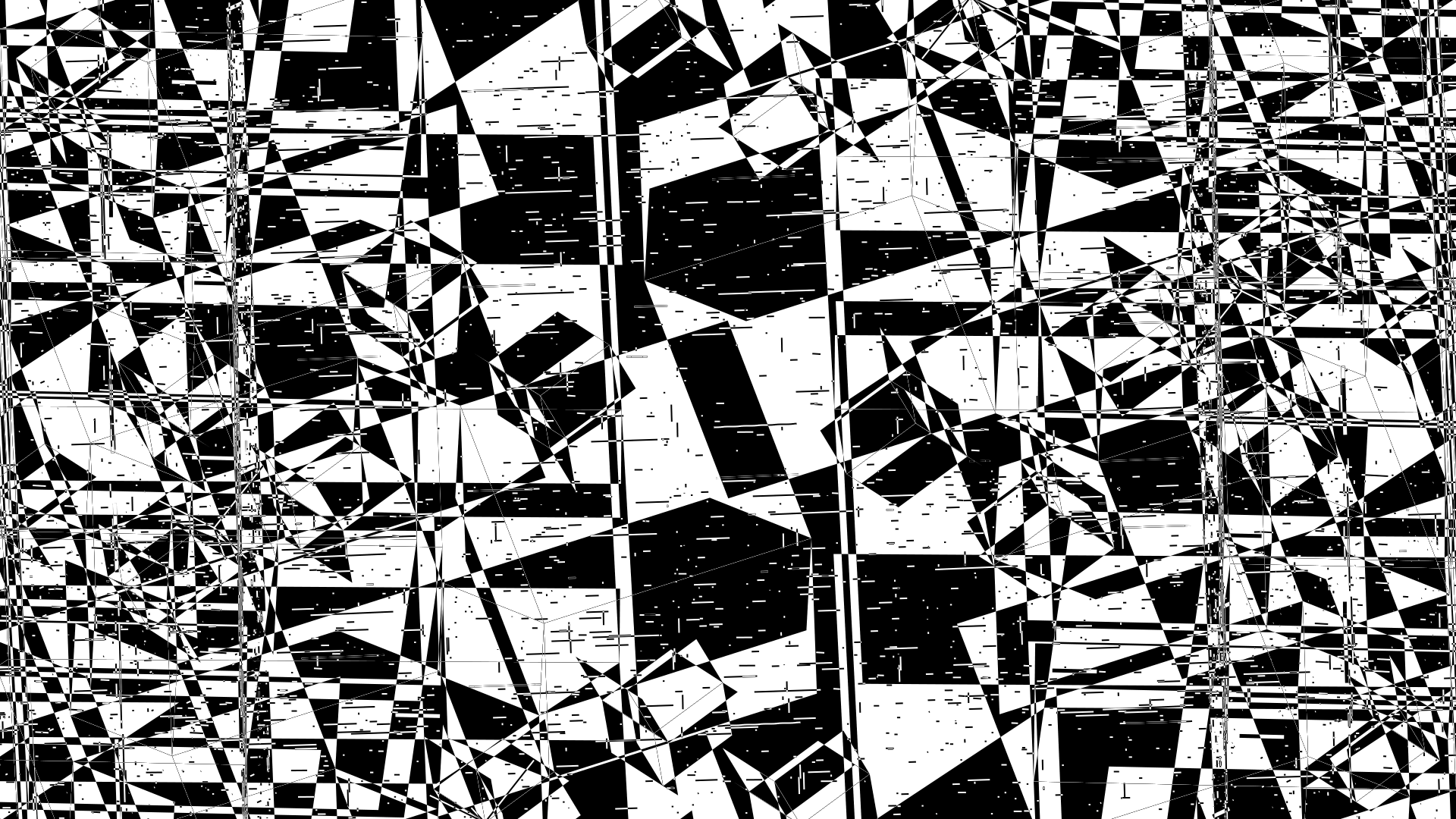
c c[1-8] a [xy][yzwvu] astep-vfast
c c[5-8] f . s5cs
rotthis3
rep 5
`e` = 0.04 `z` = 1.00
`e` = 0.04 `z` = 1.00
`e` = 0.01 `z` = 1.00
`e` = 0.00 `z` = 1.00
The Ascent video released as a black-and-white version, which is the source of the frames you've seen in this walkthrough.
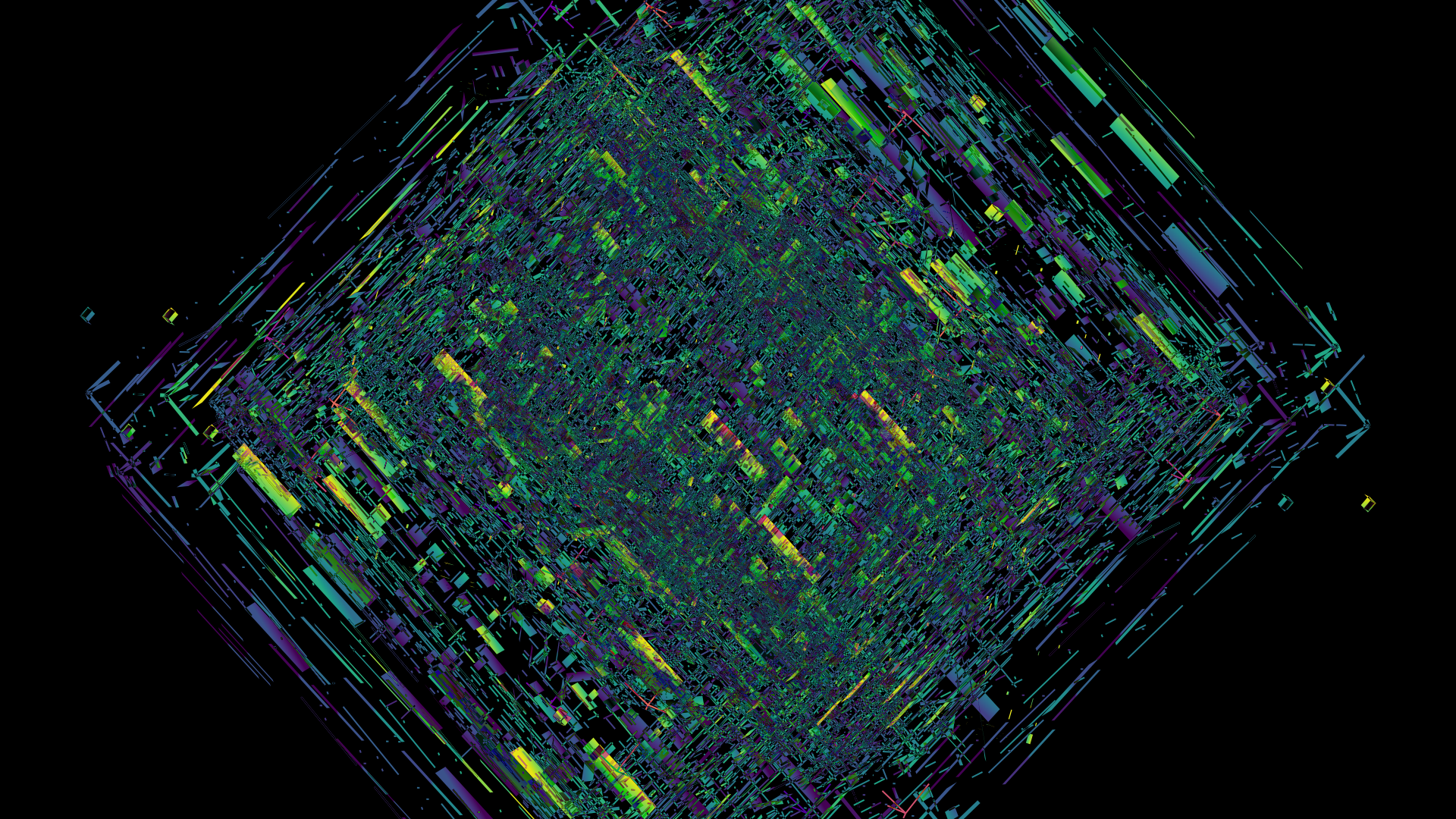
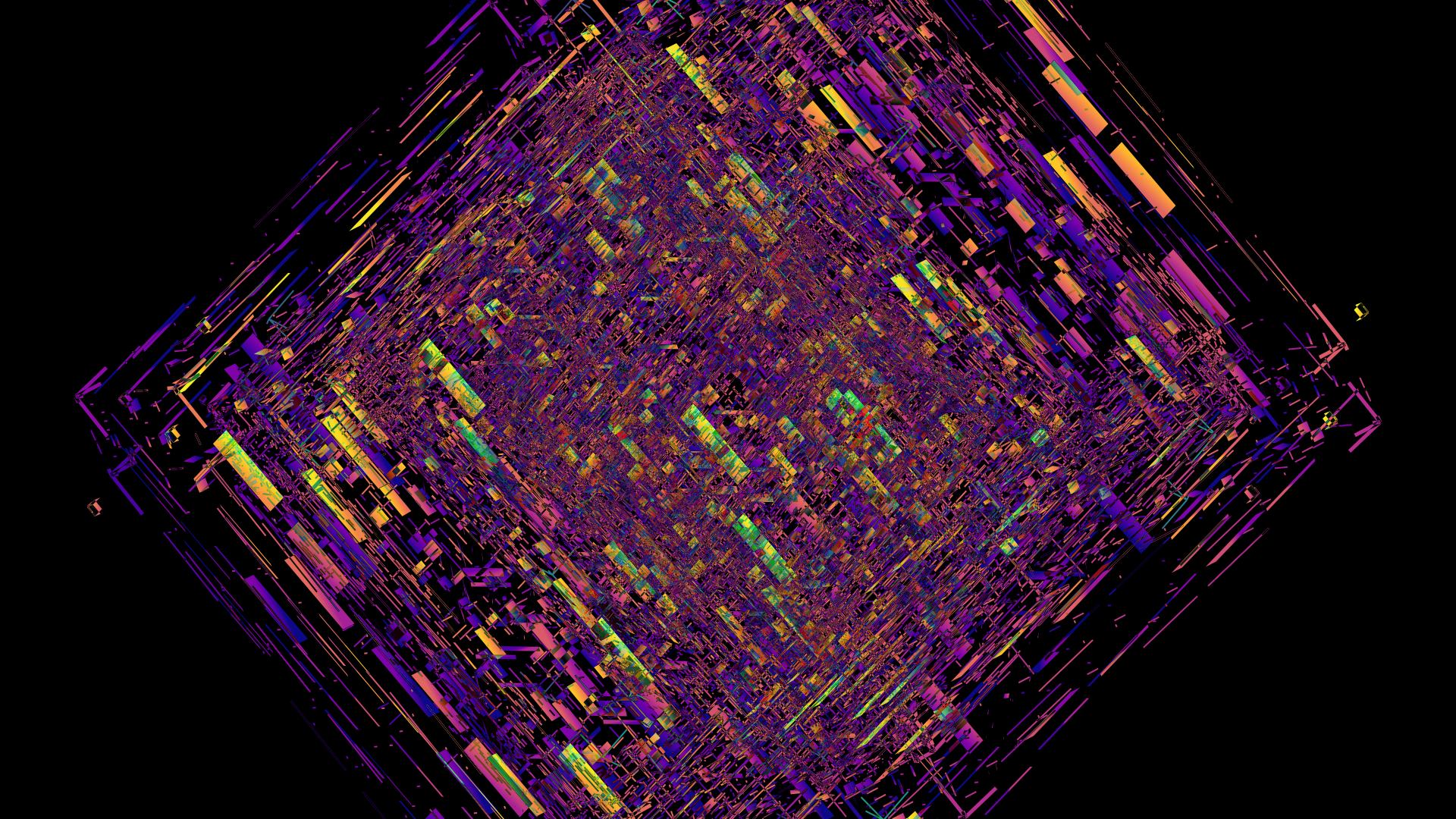
There are two more versions of the video — one using the viridis (yellow, green, blue, purple) color scheme and the other using plasma (yellow, orange, red, pruple, violet).
The color encodes the z-distance (into the screen) to the element.
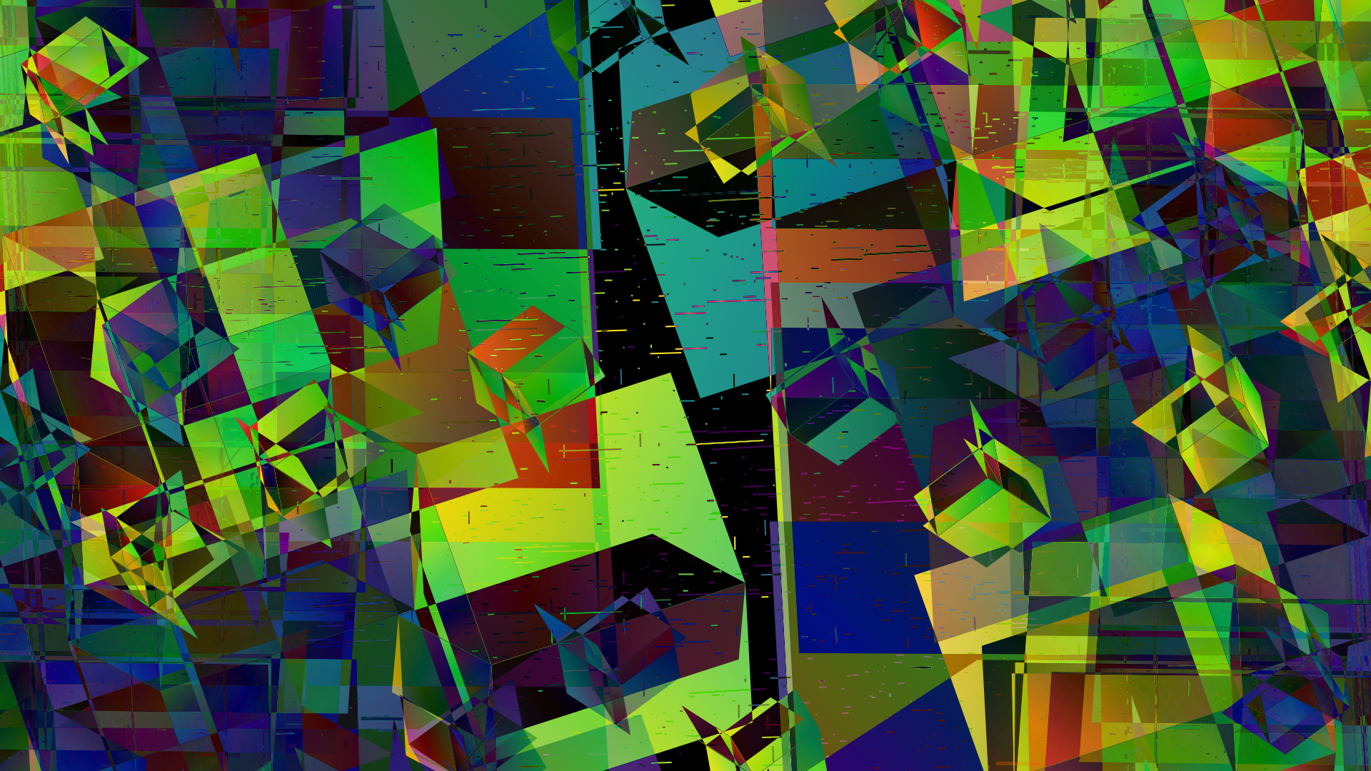
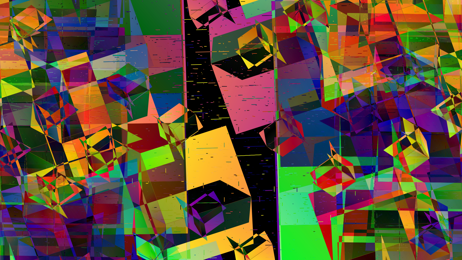
At around 4 minutes into the video, the entire scene appears to reset. This is achieved by slowly resetting the scene angle to a specific point of view — don't ask me how long it took to find it.
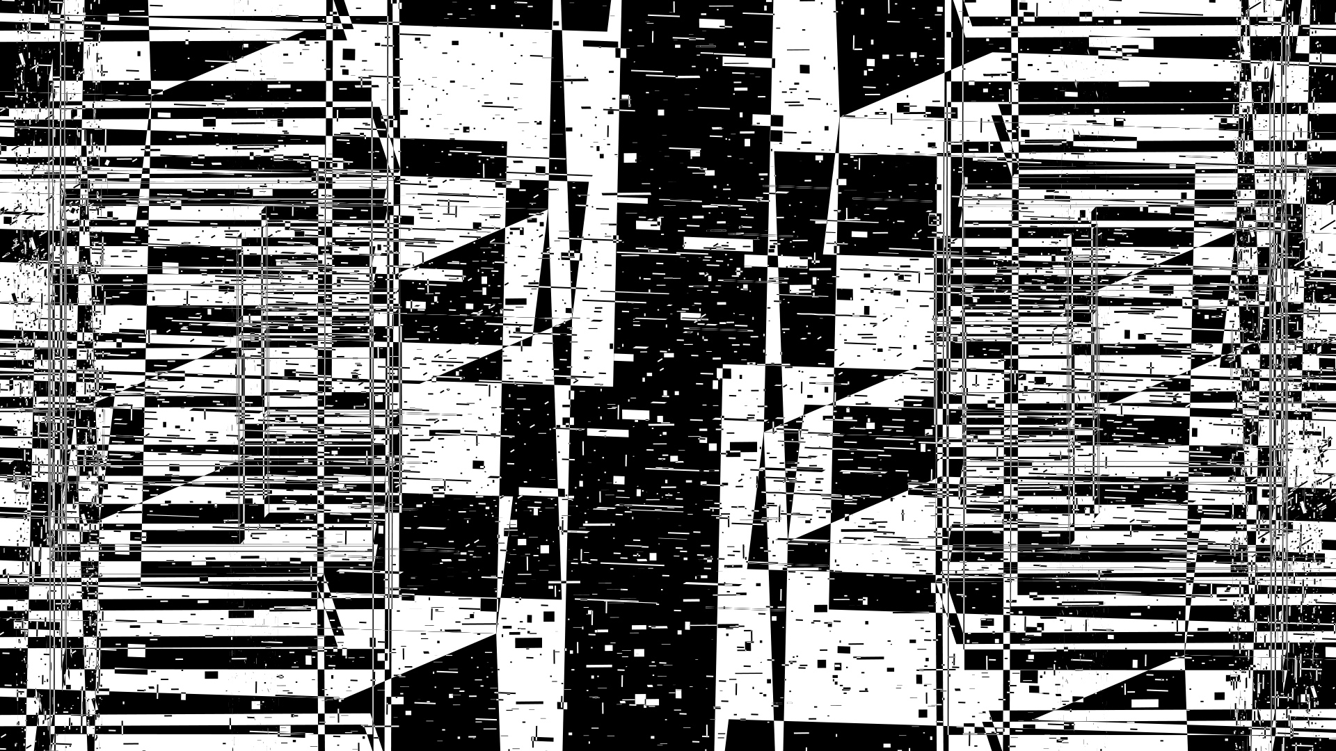
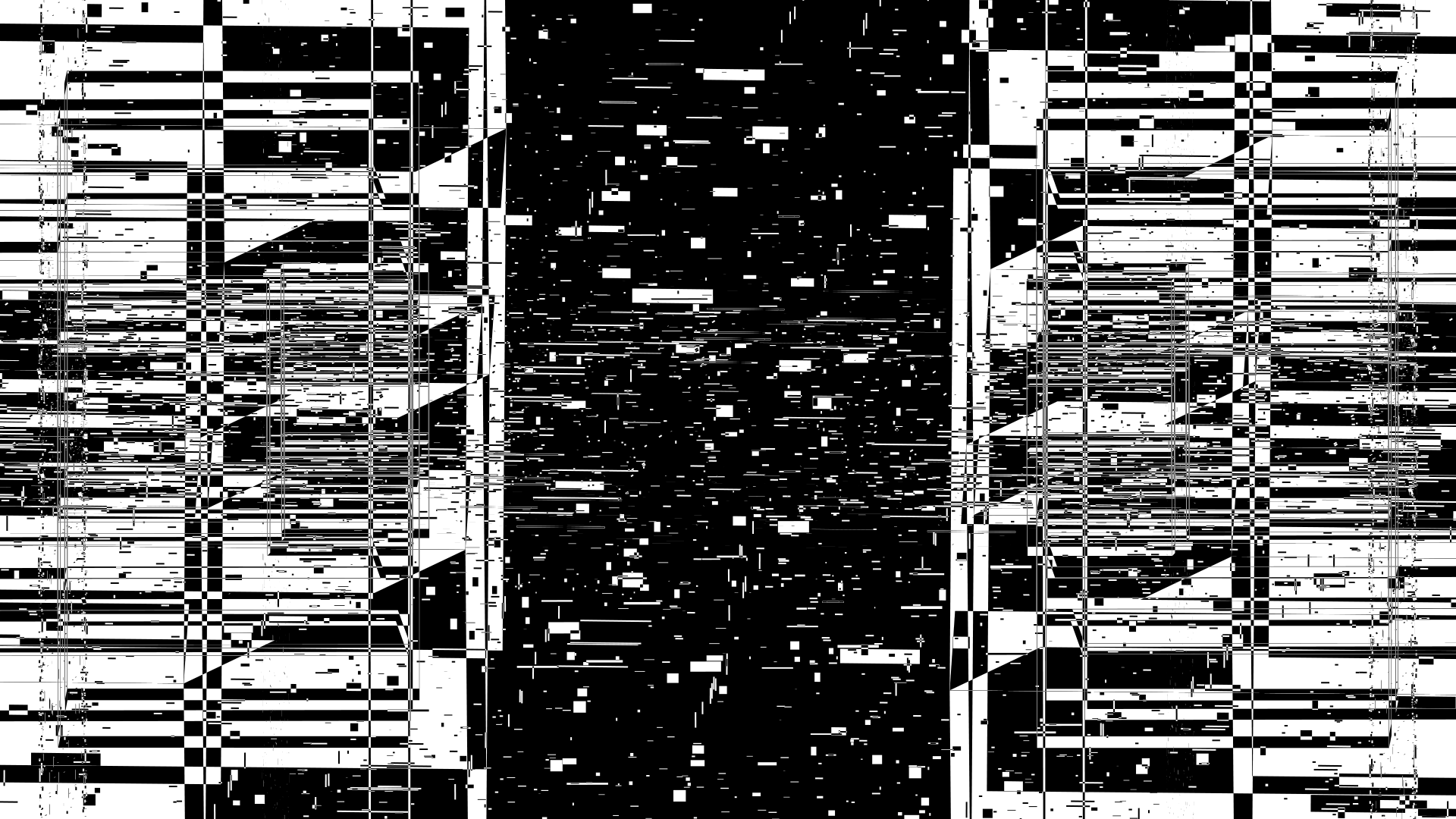
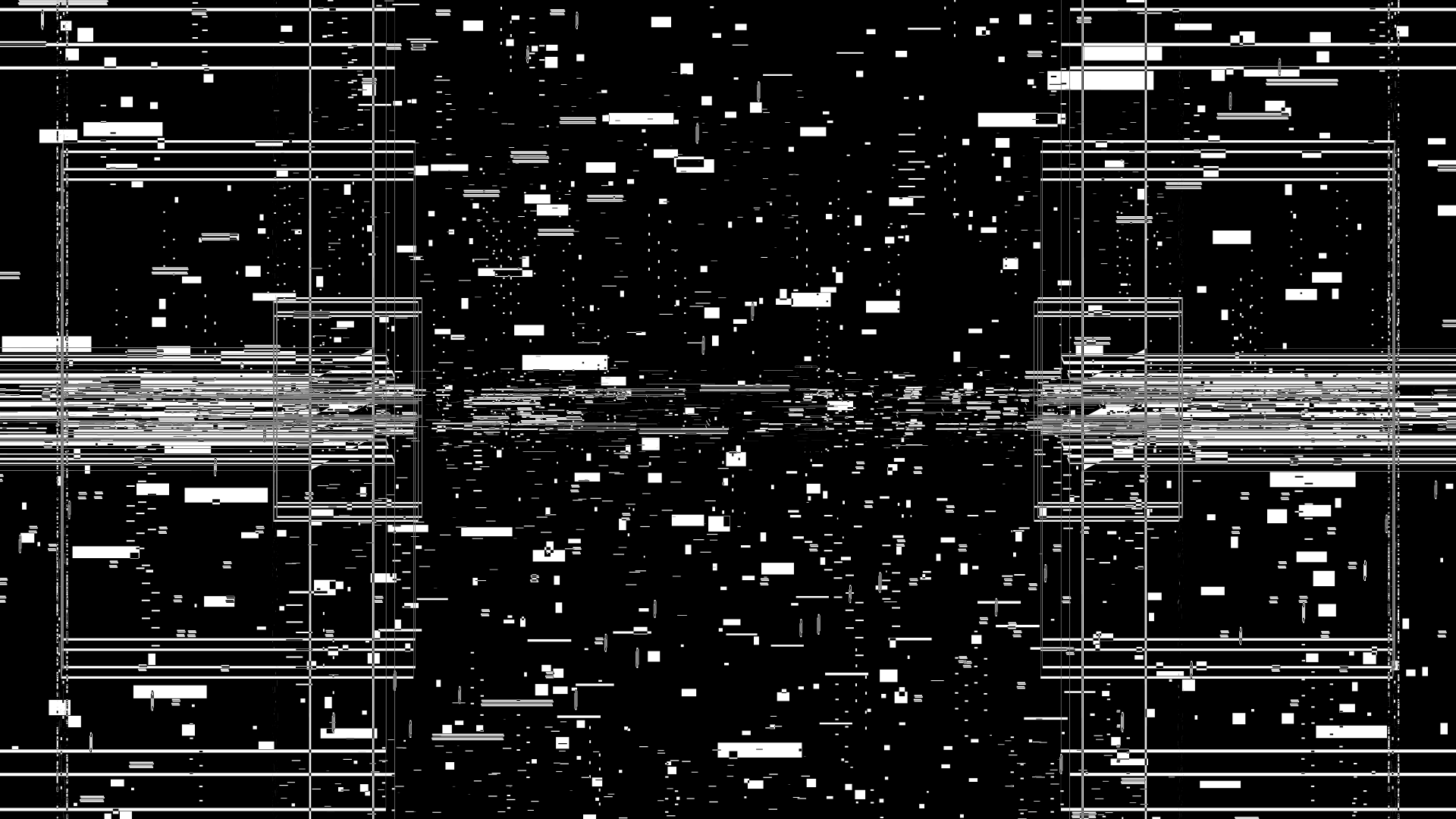
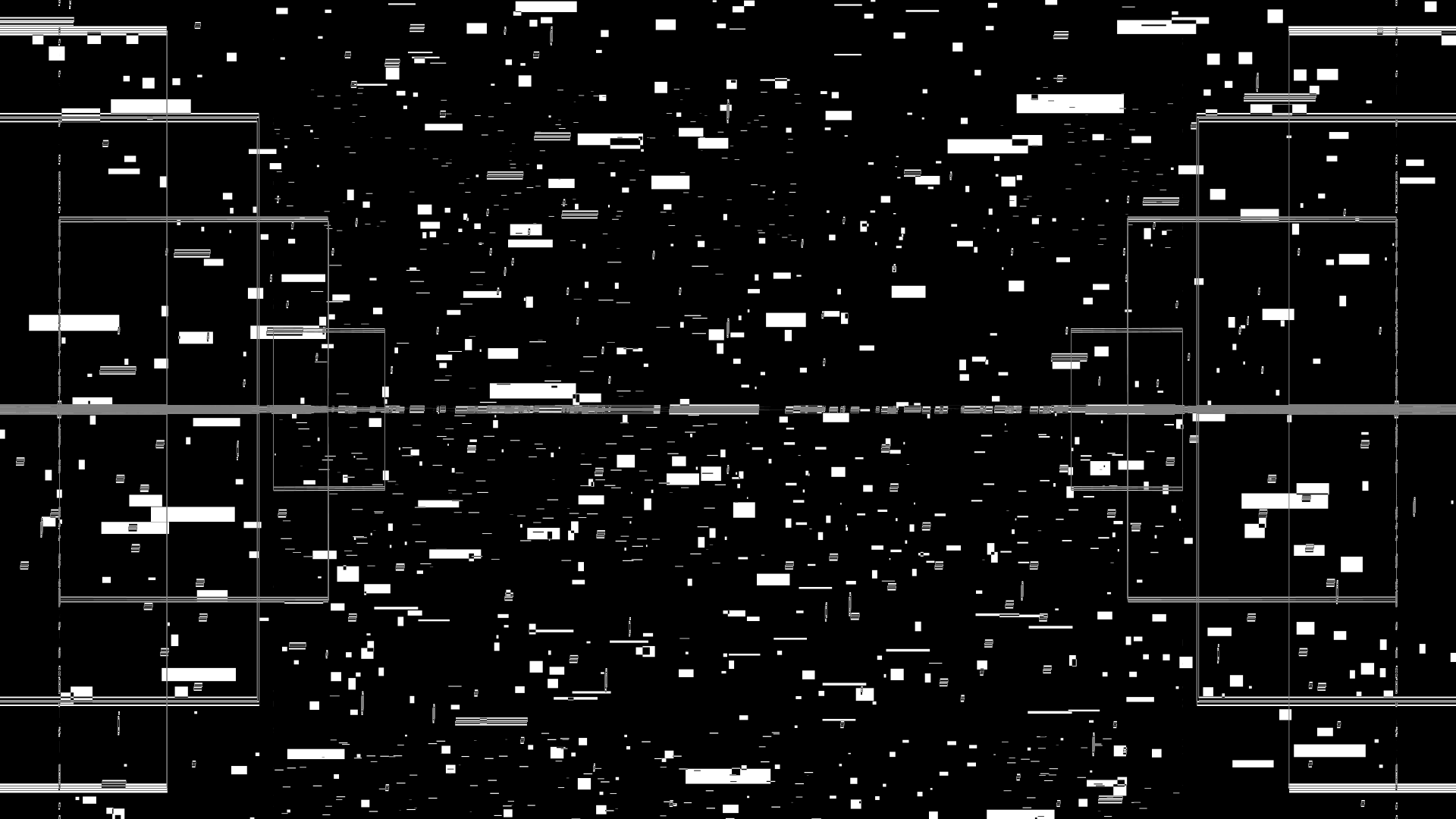
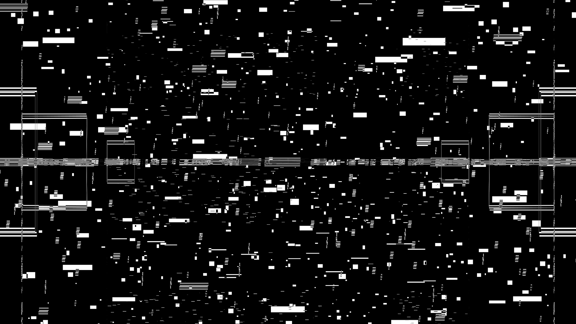
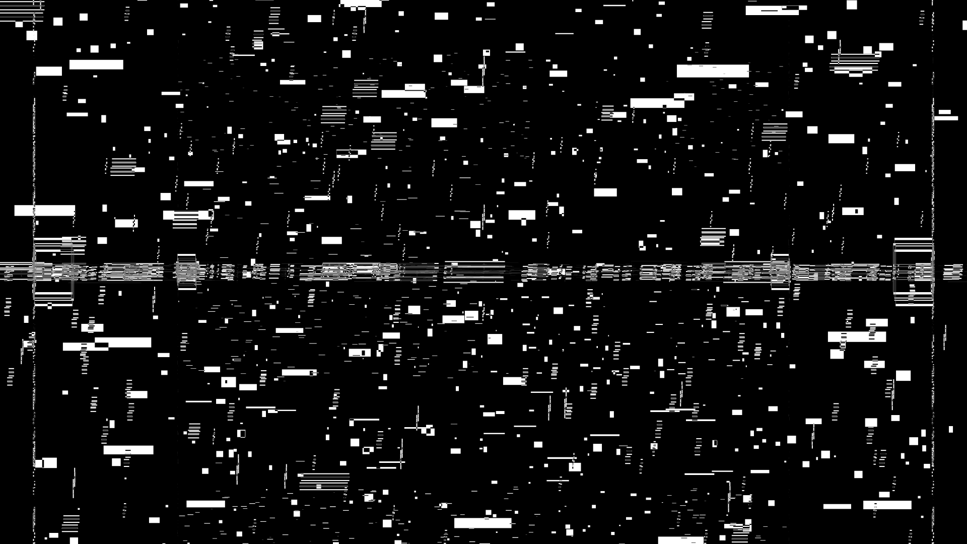
The angles of all cubes are either zero or 180 and the scene is rotated so that what we see is a pretty minimal projection.
You'll notice that 5 new cubes Ca—Cd have been introduced. These have maps for 22/7 and 179/57, which are starting to grow. The elements for these maps are drawn as filled rectangles instead of just outlines.

a xv refxv
a xw refxw
a xy refxy
a xz refxz
a yv refyv
a yw refyw
a yz refyz
c c[0-9a-d] a . 0
map_fade(c[a-d],.,ps6)
a xw d0.01
cube c[0-8] fade . ps15
cube_rot(.,[xy][yzwvu],astep-vvslow)
f . . map . fade ps15
rot6vvs
size . ps20
`e` = 0.04 `z` = 1.00
`e` = 0.04 `z` = 1.00
`e` = 0.01 `z` = 1.00
`e` = 0.00 `z` = 1.00
`e` = 0.01 `z` = 1.00
`e` = 0.01 `z` = 1.00
`e` = 0.01 `z` = 1.00
`e` = 0.01 `z` = 1.00
The scene starts to unravel and the rectangles of the area maps start to look like falling snow.
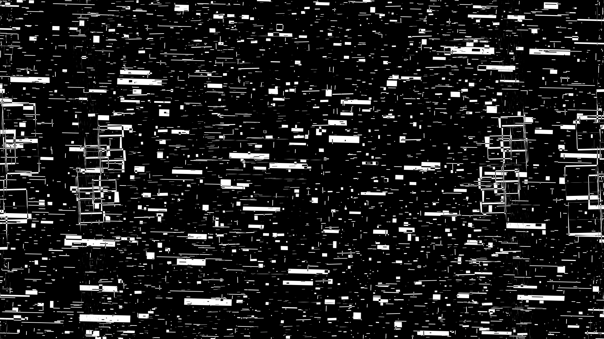
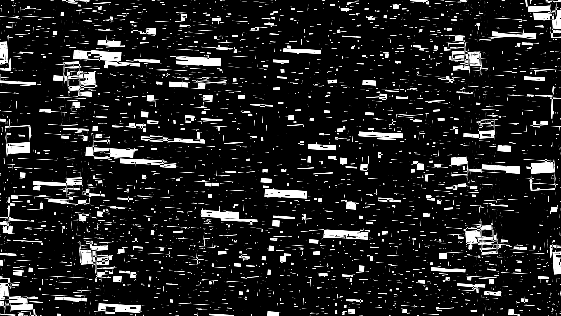
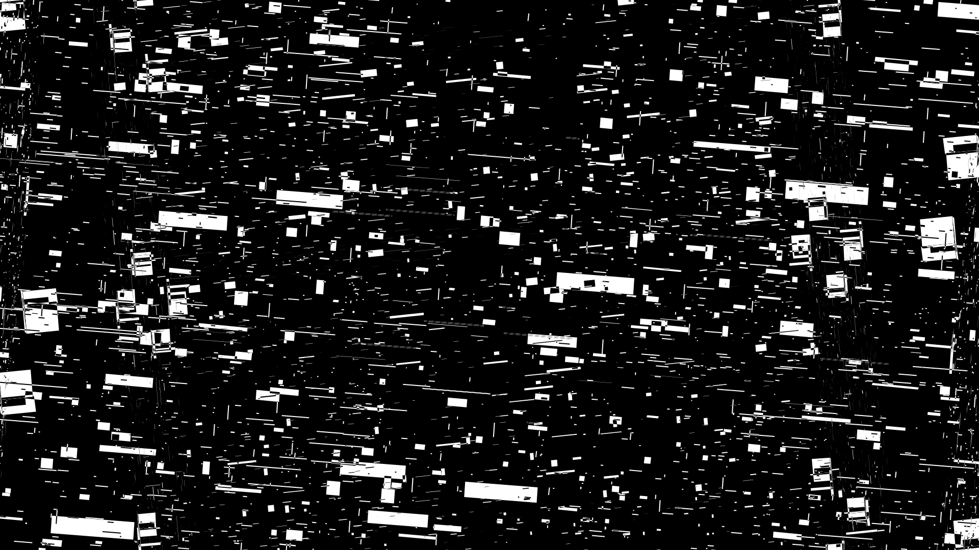
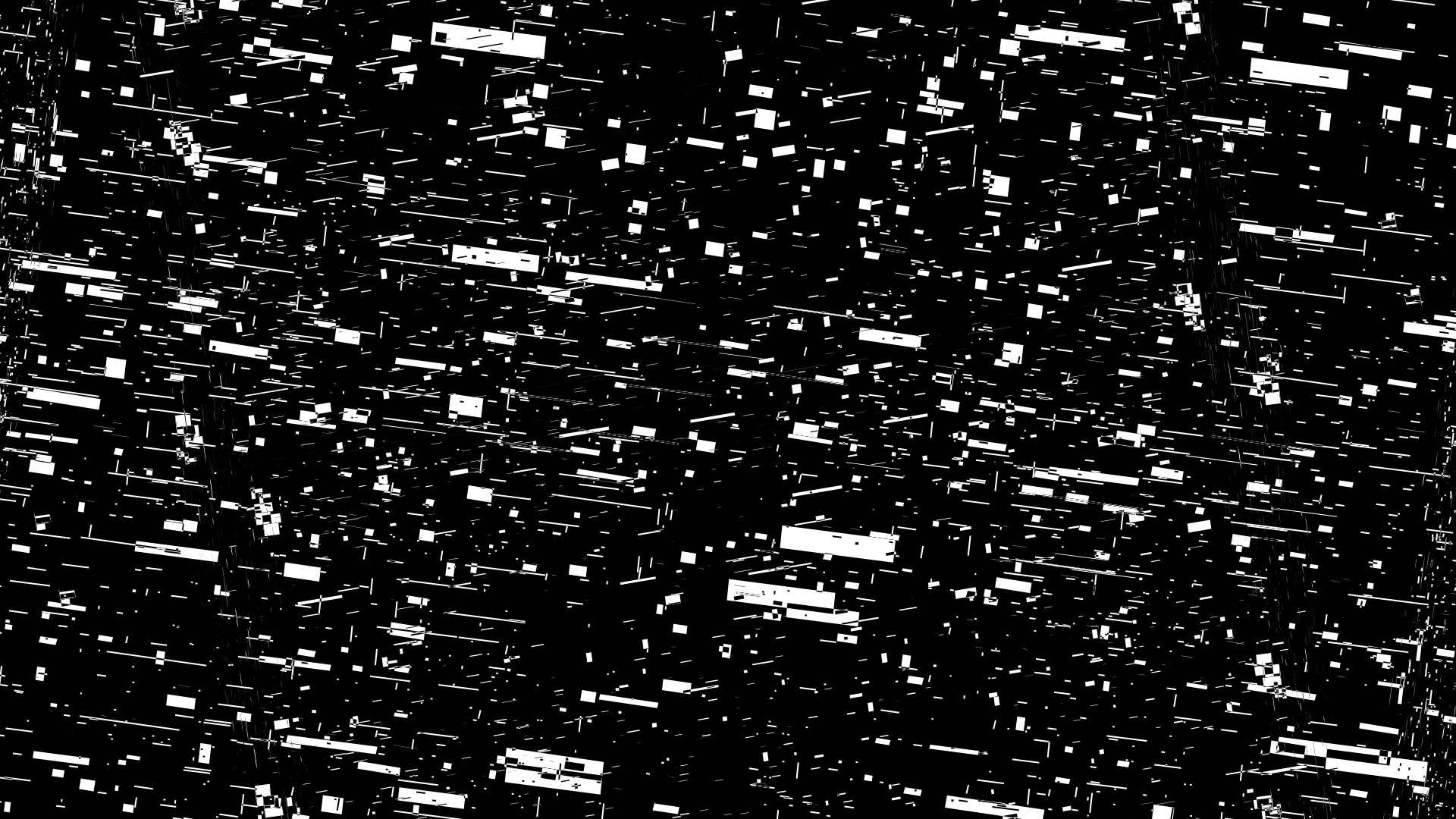
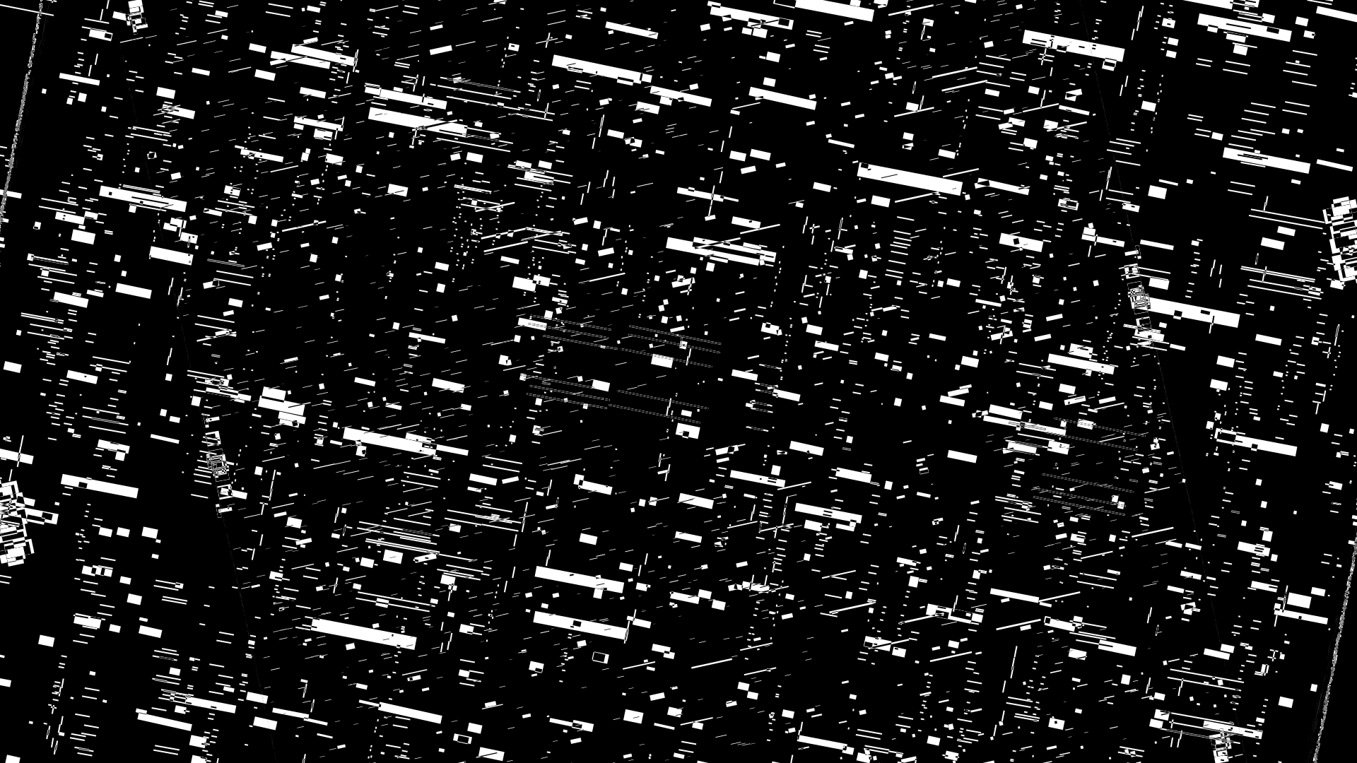
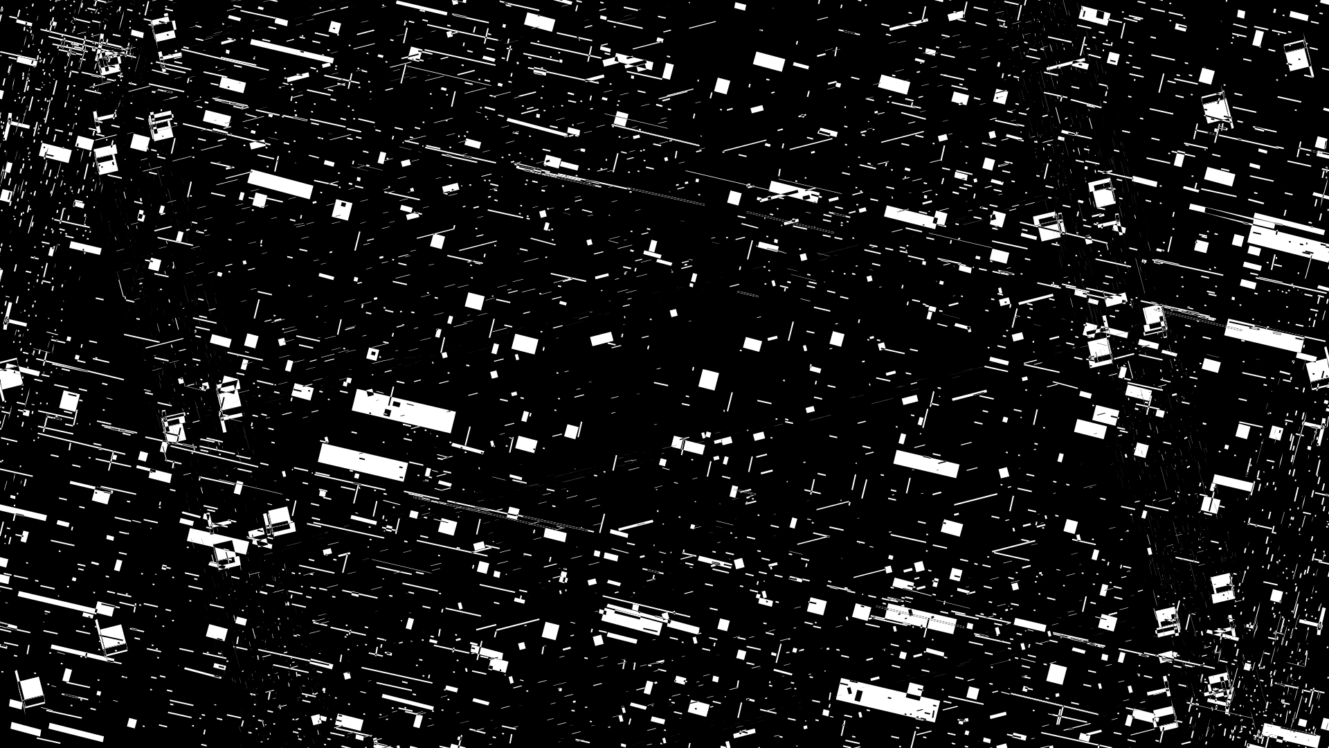
This part of the video looks particularly warm and inviting when rendered in color.
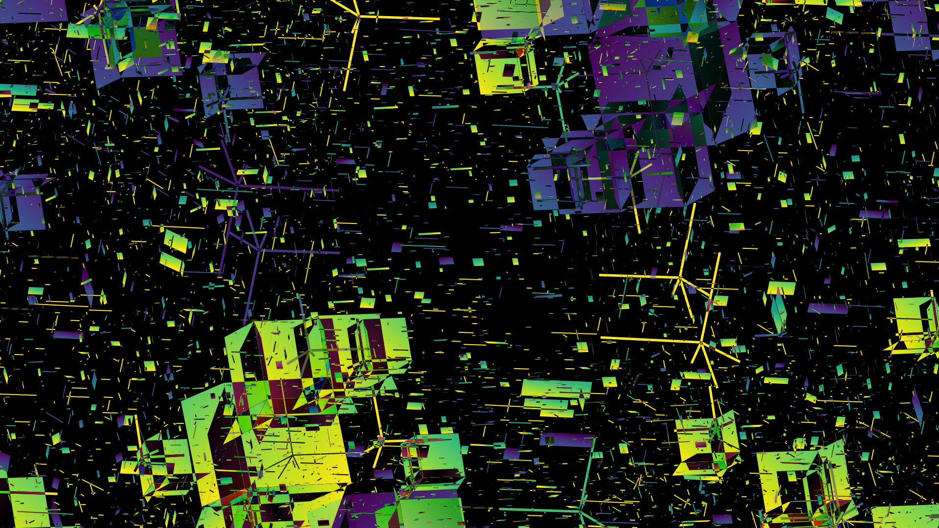
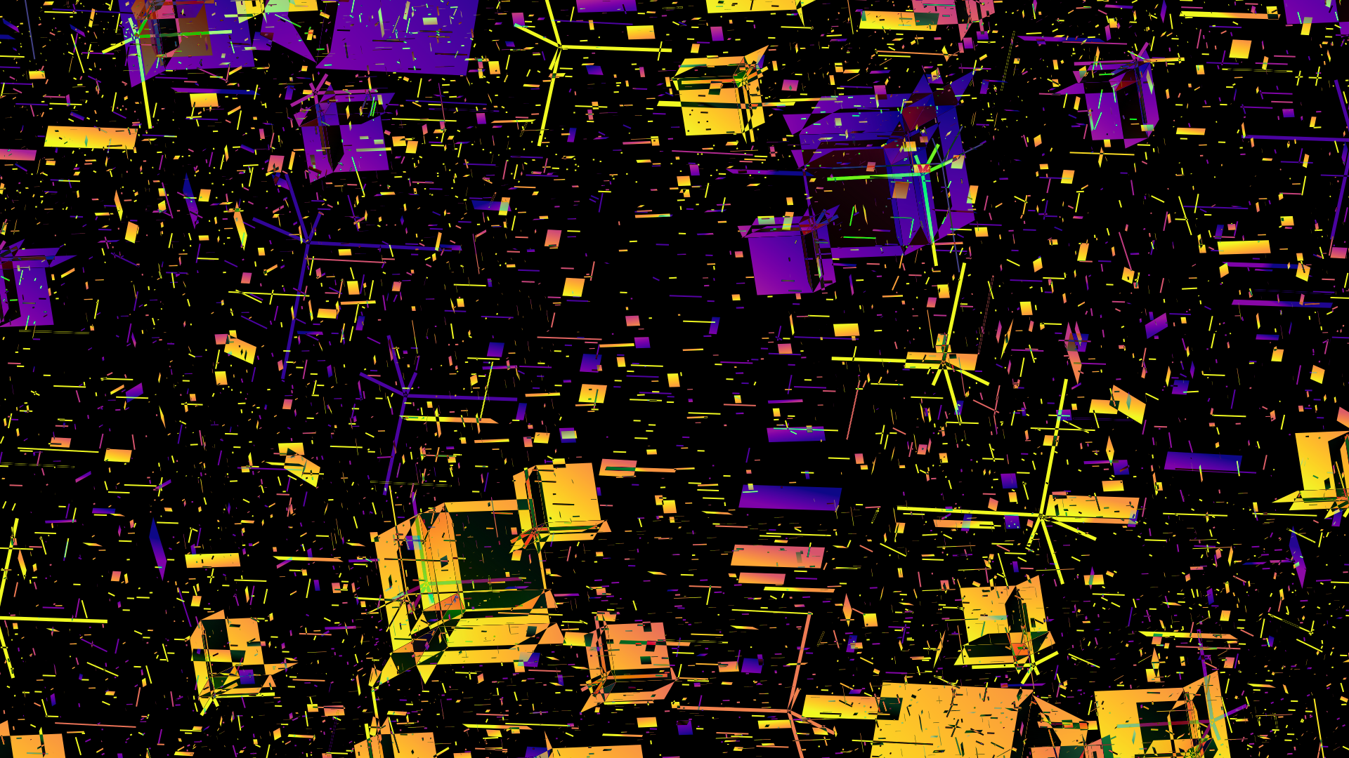
The last 4 cubes are introduced: Ce–Ch. These have area maps of the digits of `\pi`, which are also drawn as filled rectangles. Notice that when a cube's edge parameter is zero `e = 0` the cube itself isn't drawn but area map projections on its faces can appear if the maps' `e>0`.
cube c[0-2] fade . p5
cube_rot(.,[xy][yzwvu],astep-med)
face c[0-9a-e] . map . fade p5
rot6f
rep 2
`e` = 0.06 `z` = 1.00
`e` = 0.06 `z` = 1.00
`e` = 0.03 `z` = 1.00
`e` = 0.02 `z` = 1.00
`e` = 0.03 `z` = 1.00
`e` = 0.03 `z` = 1.00
`e` = 0.03 `z` = 1.00
`e` = 0.03 `z` = 1.00
`e` = 0.02 `z` = 1.00
`e` = 0.00 `z` = 1.00
`e` = 0.00 `z` = 1.00
`e` = 0.00 `z` = 1.00
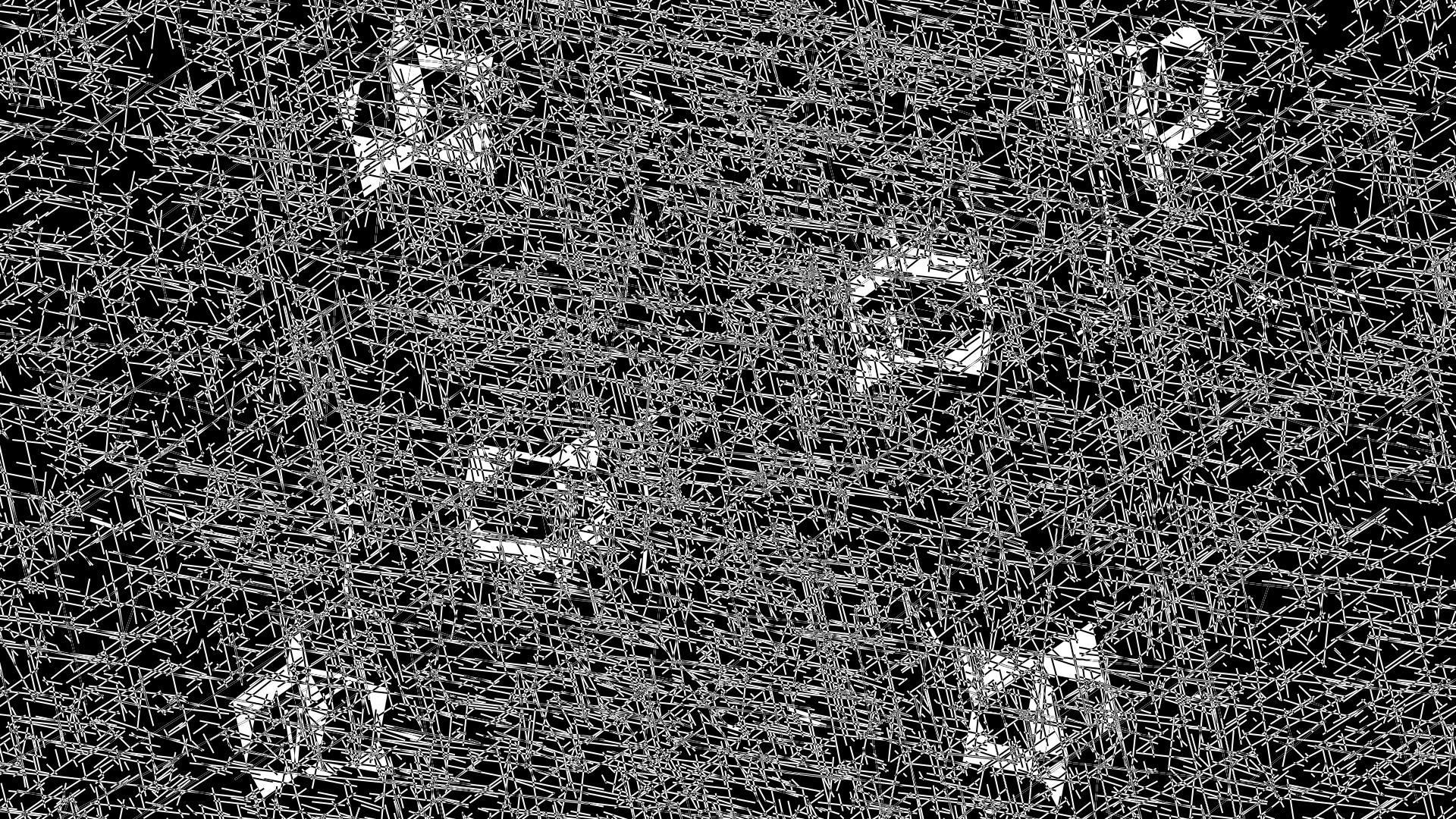
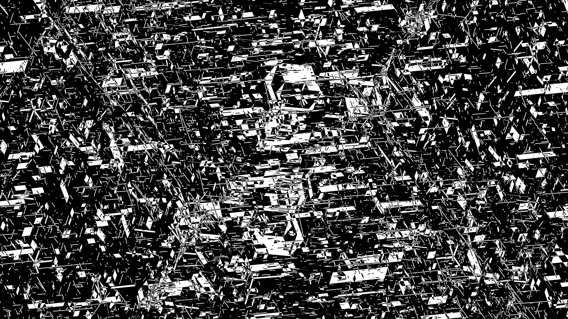
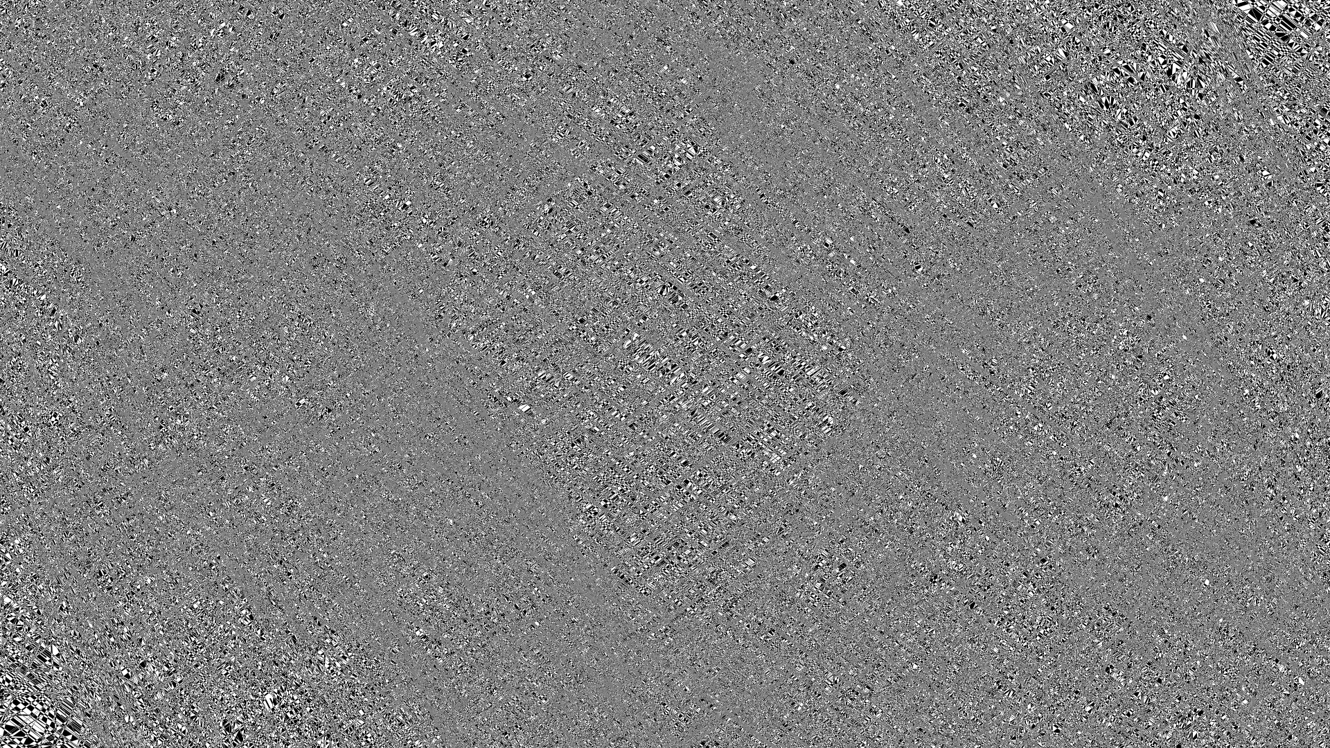
For the climax, everything that's been seen so far is turned back on: edges grow, cube faces are filled and all map edges and filled rectangles grow. All the elements are rendered with difference blend (i.e. black on black gives white, white on white gives black) and the scene turns to noise.

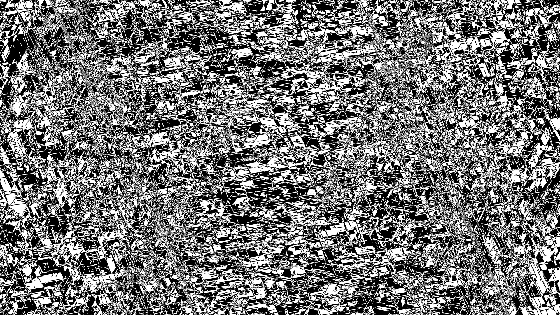
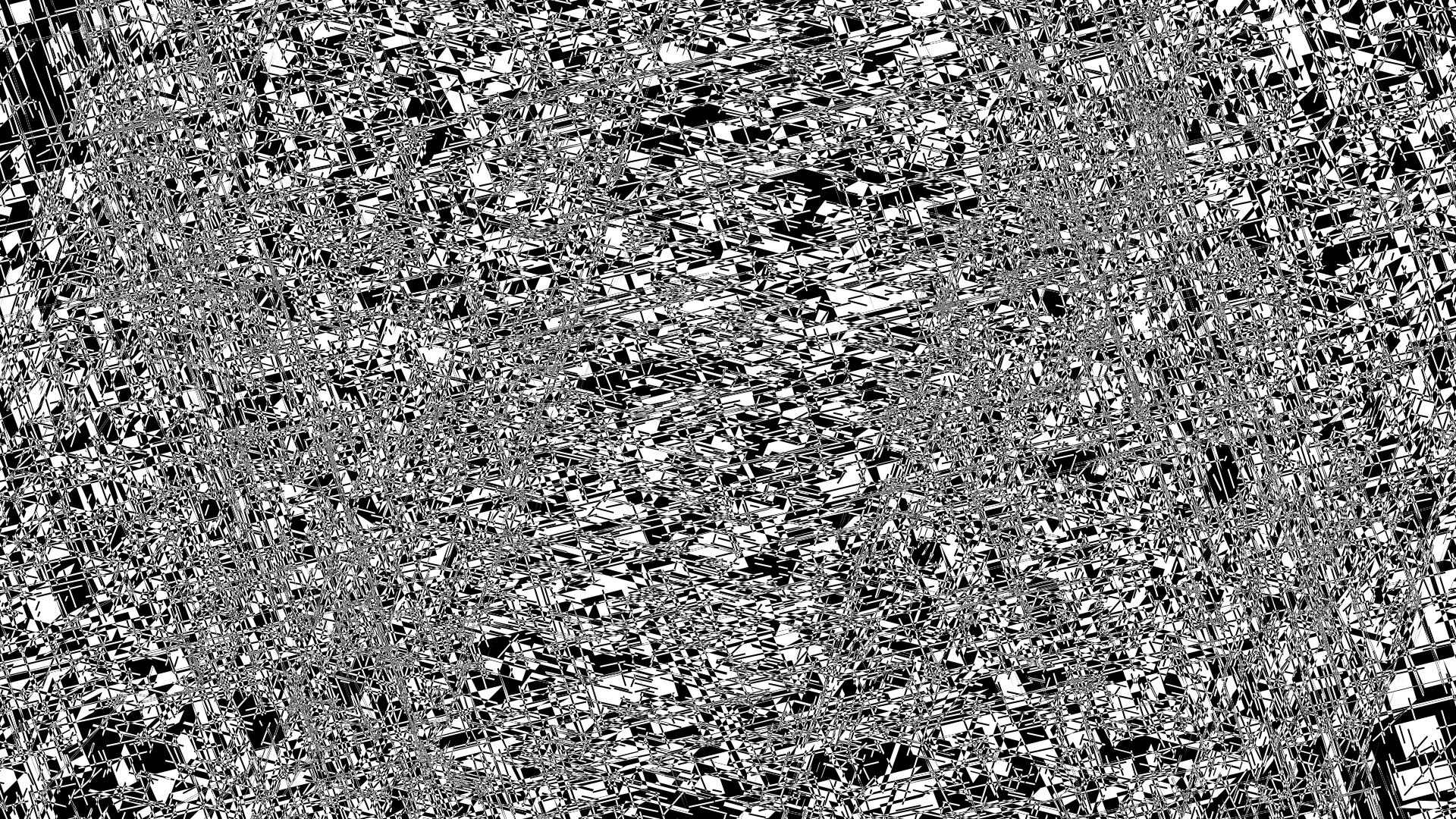
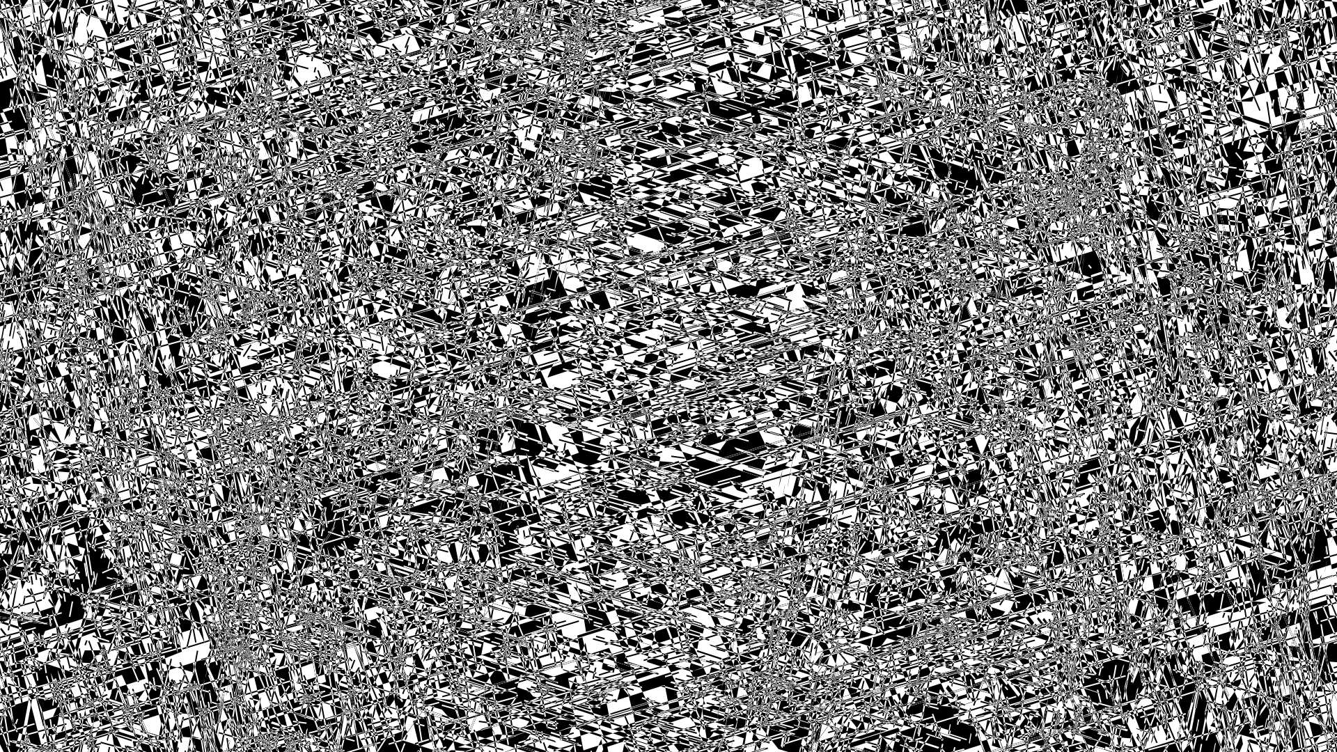
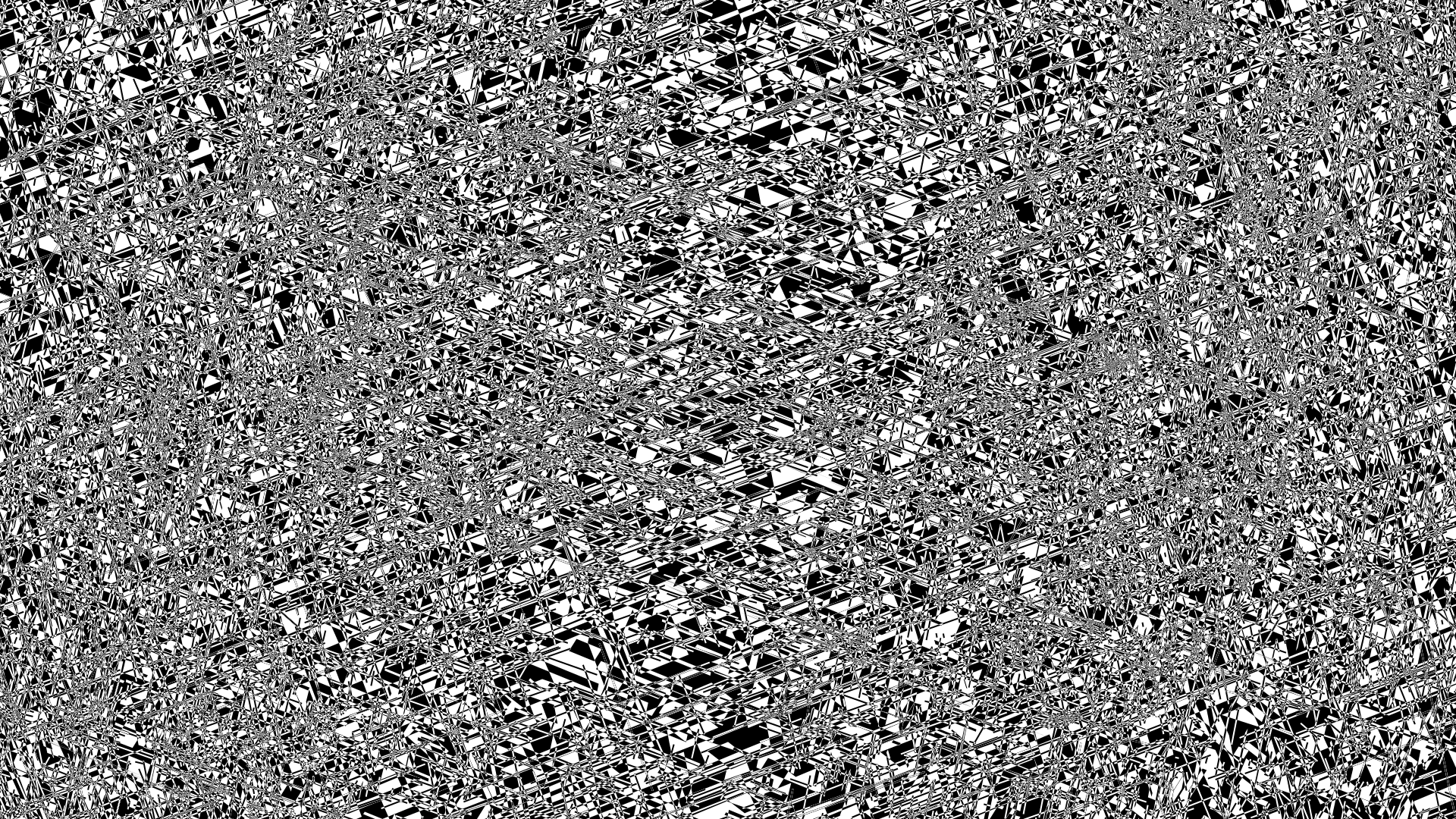
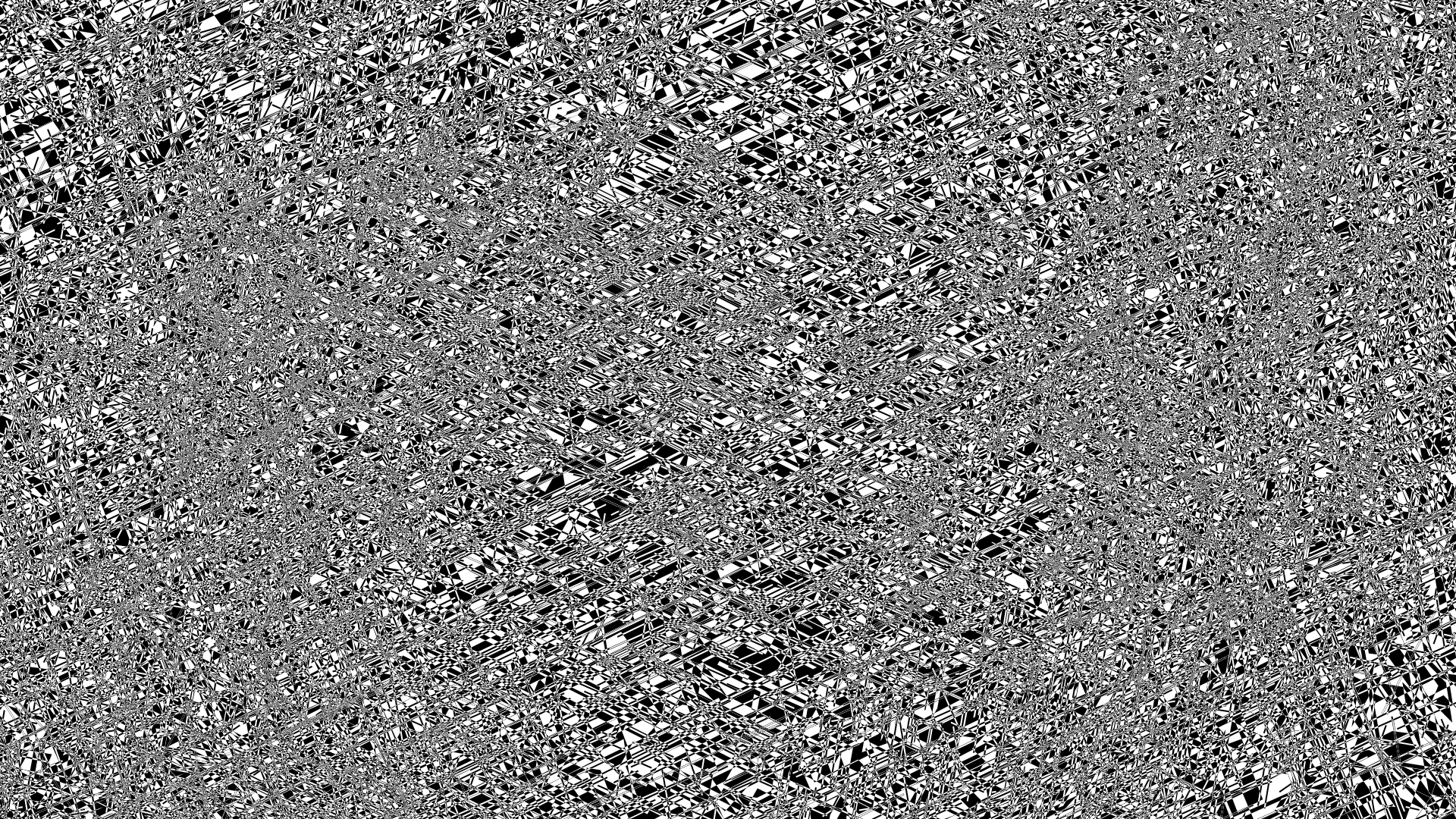
The noise builds and you get brief glimpses of thousands of edges and faces stacking into vague patterns. If you look at the cube parameters for this frame 7440, you'll notice that everything is “on”: Cubes C0–C8 have a non-zero size and non-zero edge and the remaining cubes have map edges in the interval `e = [0.18,0.41]`.
cube_rot(.,[xy][yzwvu],astep-med)
rot6vf
rep 2
`e` = 0.43 `z` = 1.00
`e` = 0.43 `z` = 1.00
`e` = 0.41 `z` = 1.00
`e` = 0.40 `z` = 1.00
`e` = 0.41 `z` = 1.00
`e` = 0.41 `z` = 1.00
`e` = 0.41 `z` = 1.00
`e` = 0.41 `z` = 1.00
`e` = 0.40 `z` = 1.00
`e` = 0.34 `z` = 1.00
`e` = 0.27 `z` = 1.00
`e` = 0.18 `z` = 1.00
By about 5:20, it's time to wrap the show up. This is done by slowly zooming the camera out and shrinking the edges of all cubes and maps.
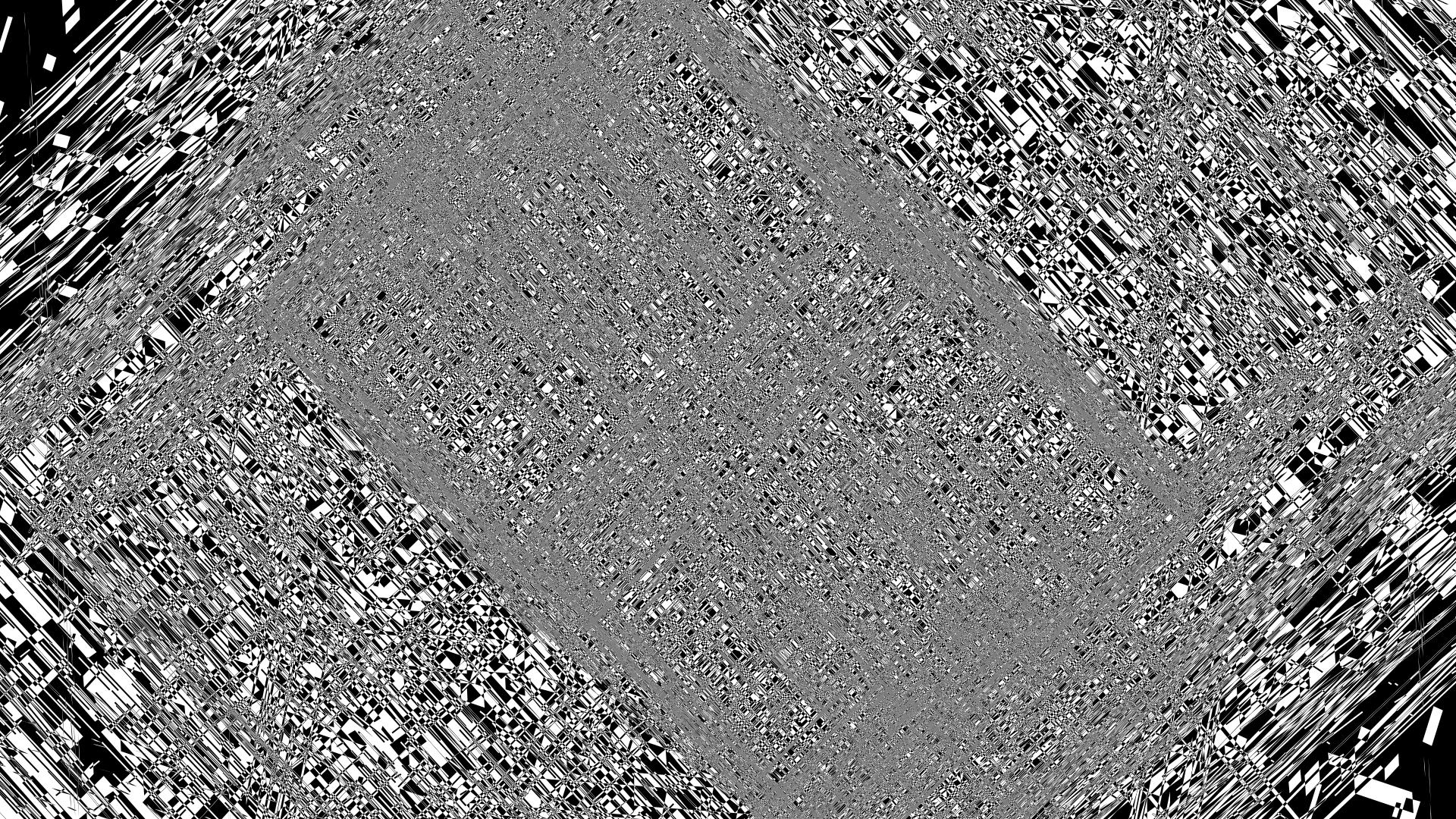
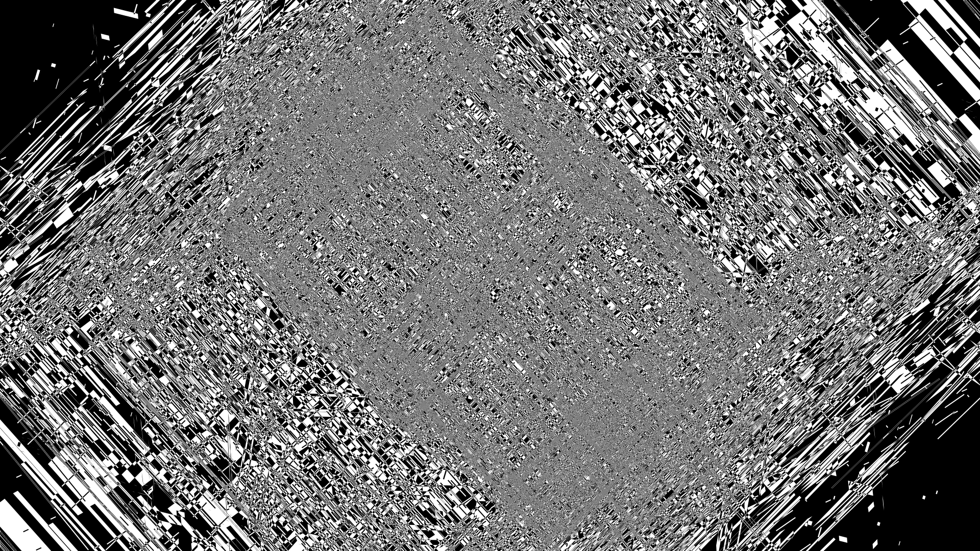
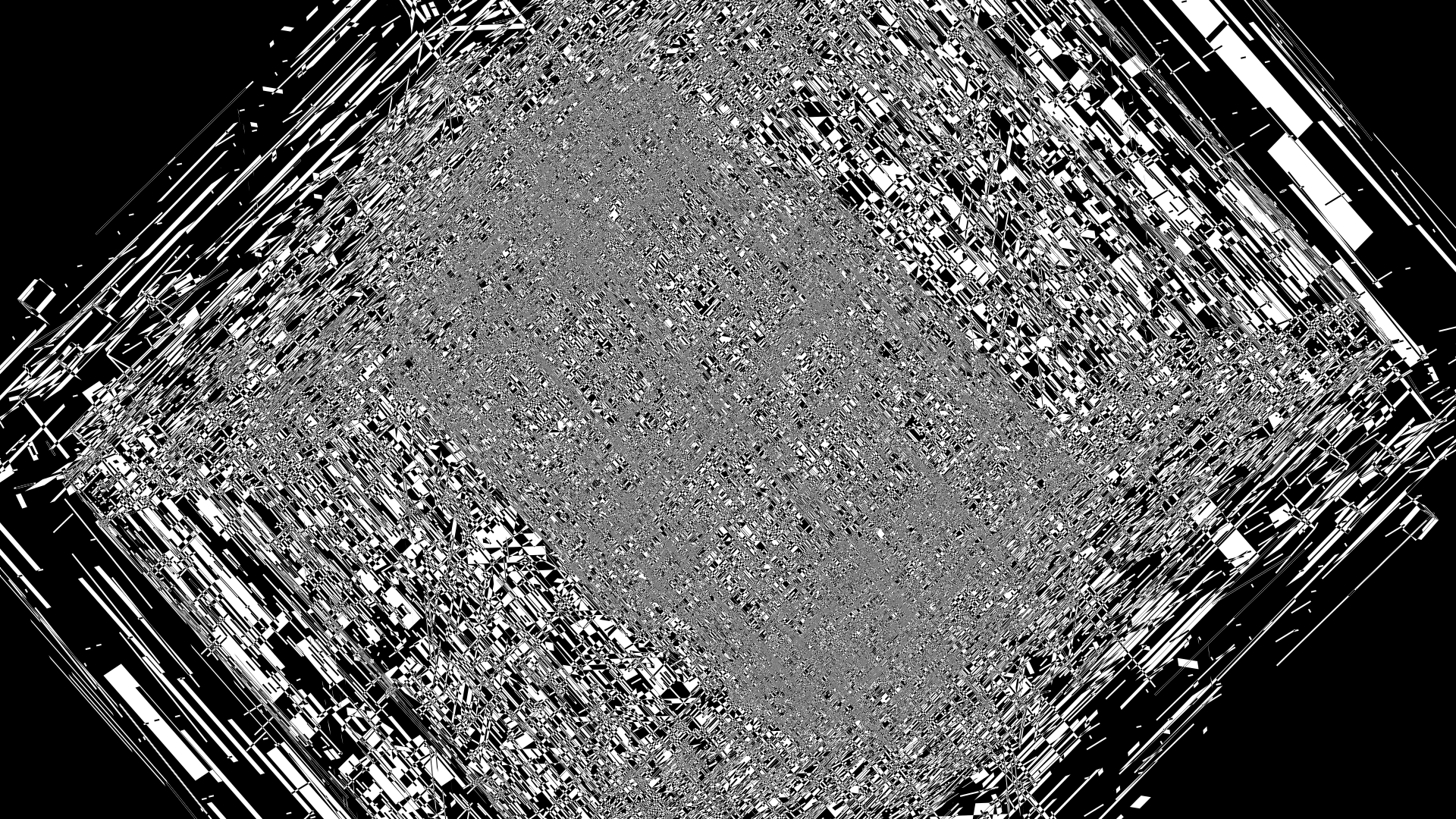
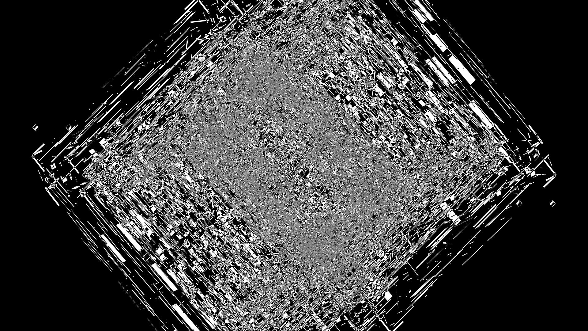
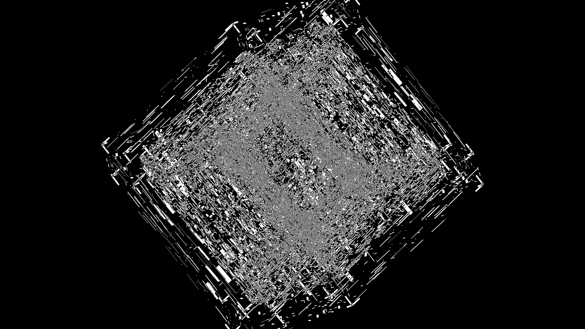
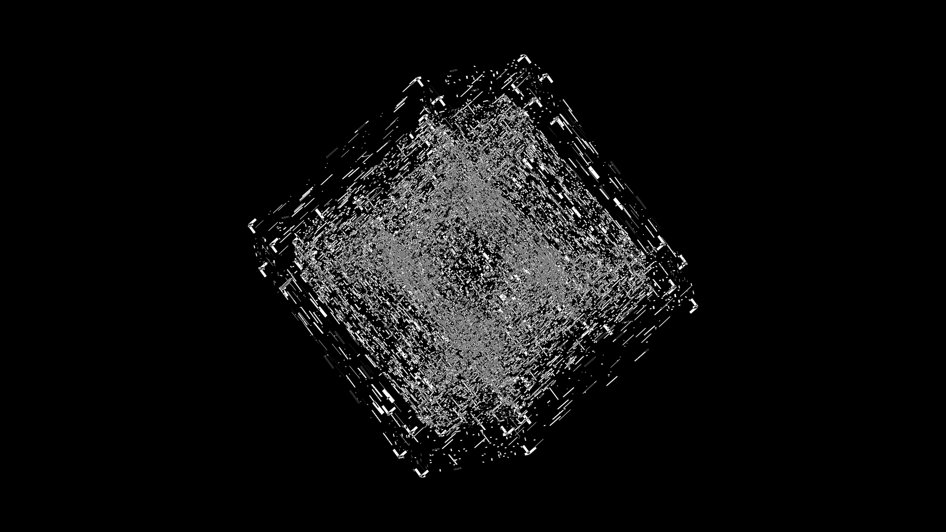
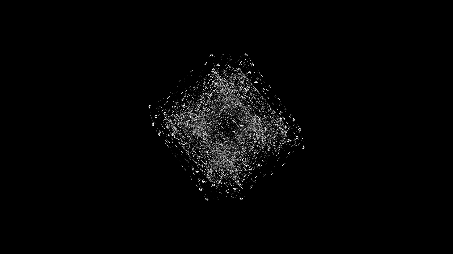
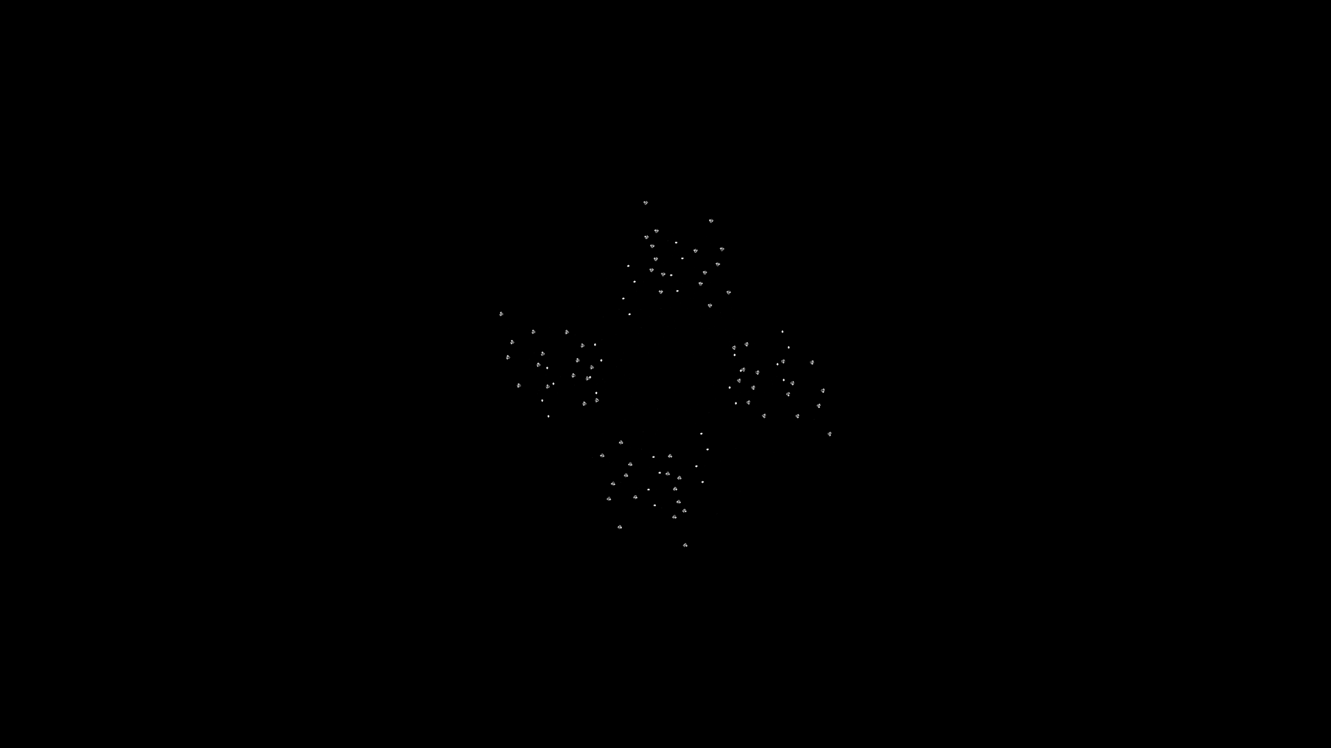
In the color versions of the video, the zoomout gives you a chance to see more details.
In this frame, one of the last where anything is visible, the zoom is `z=0.25` and cube edges are `e<0.03` and the maps have disappeared (`e=0`). Thus, what you're seeing is just the `3 \times 32 = 96` tiny vertices of cubes C0, C1 and C2.

cube . f . q50
cube_rot(.,[xy][ywvu],astep-med)
map_fade(.,.,q50)
rot6s
size . q30
rep 6
`e` = 0.00 `z` = 1.00
`e` = 0.00 `z` = 1.00
`e` = 0.00 `z` = 1.00
`e` = 0.00 `z` = 1.00
`e` = 0.00 `z` = 1.00
`e` = 0.00 `z` = 1.00
`e` = 0.00 `z` = 1.00
`e` = 0.00 `z` = 1.00
`e` = 0.00 `z` = 1.00
`e` = 0.00 `z` = 1.00
`e` = 0.00 `z` = 1.00
`e` = 0.00 `z` = 1.00
A second later, everything is gone.
Beyond Belief Campaign BRCA Art
Fuelled by philanthropy, findings into the workings of BRCA1 and BRCA2 genes have led to groundbreaking research and lifesaving innovations to care for families facing cancer.
This set of 100 one-of-a-kind prints explore the structure of these genes. Each artwork is unique — if you put them all together, you get the full sequence of the BRCA1 and BRCA2 proteins.
Propensity score weighting
The needs of the many outweigh the needs of the few. —Mr. Spock (Star Trek II)
This month, we explore a related and powerful technique to address bias: propensity score weighting (PSW), which applies weights to each subject instead of matching (or discarding) them.
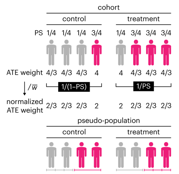
Kurz, C.F., Krzywinski, M. & Altman, N. (2025) Points of significance: Propensity score weighting. Nat. Methods 22:1–3.
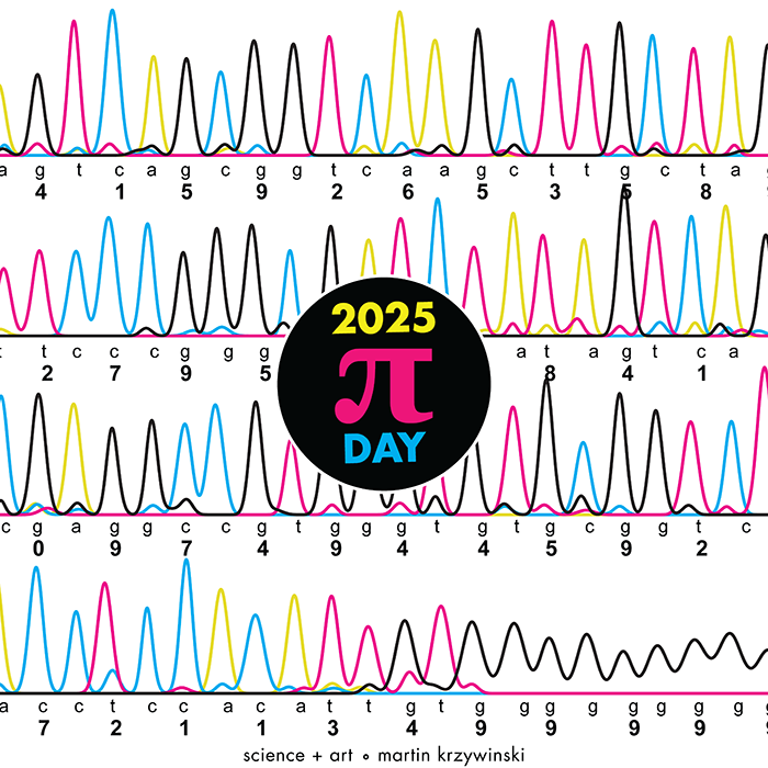
Happy 2025 π Day—
TTCAGT: a sequence of digits
Celebrate π Day (March 14th) and sequence digits like its 1999. Let's call some peaks.
Crafting 10 Years of Statistics Explanations: Points of Significance
I don’t have good luck in the match points. —Rafael Nadal, Spanish tennis player
Points of Significance is an ongoing series of short articles about statistics in Nature Methods that started in 2013. Its aim is to provide clear explanations of essential concepts in statistics for a nonspecialist audience. The articles favor heuristic explanations and make extensive use of simulated examples and graphical explanations, while maintaining mathematical rigor.
Topics range from basic, but often misunderstood, such as uncertainty and P-values, to relatively advanced, but often neglected, such as the error-in-variables problem and the curse of dimensionality. More recent articles have focused on timely topics such as modeling of epidemics, machine learning, and neural networks.
In this article, we discuss the evolution of topics and details behind some of the story arcs, our approach to crafting statistical explanations and narratives, and our use of figures and numerical simulations as props for building understanding.
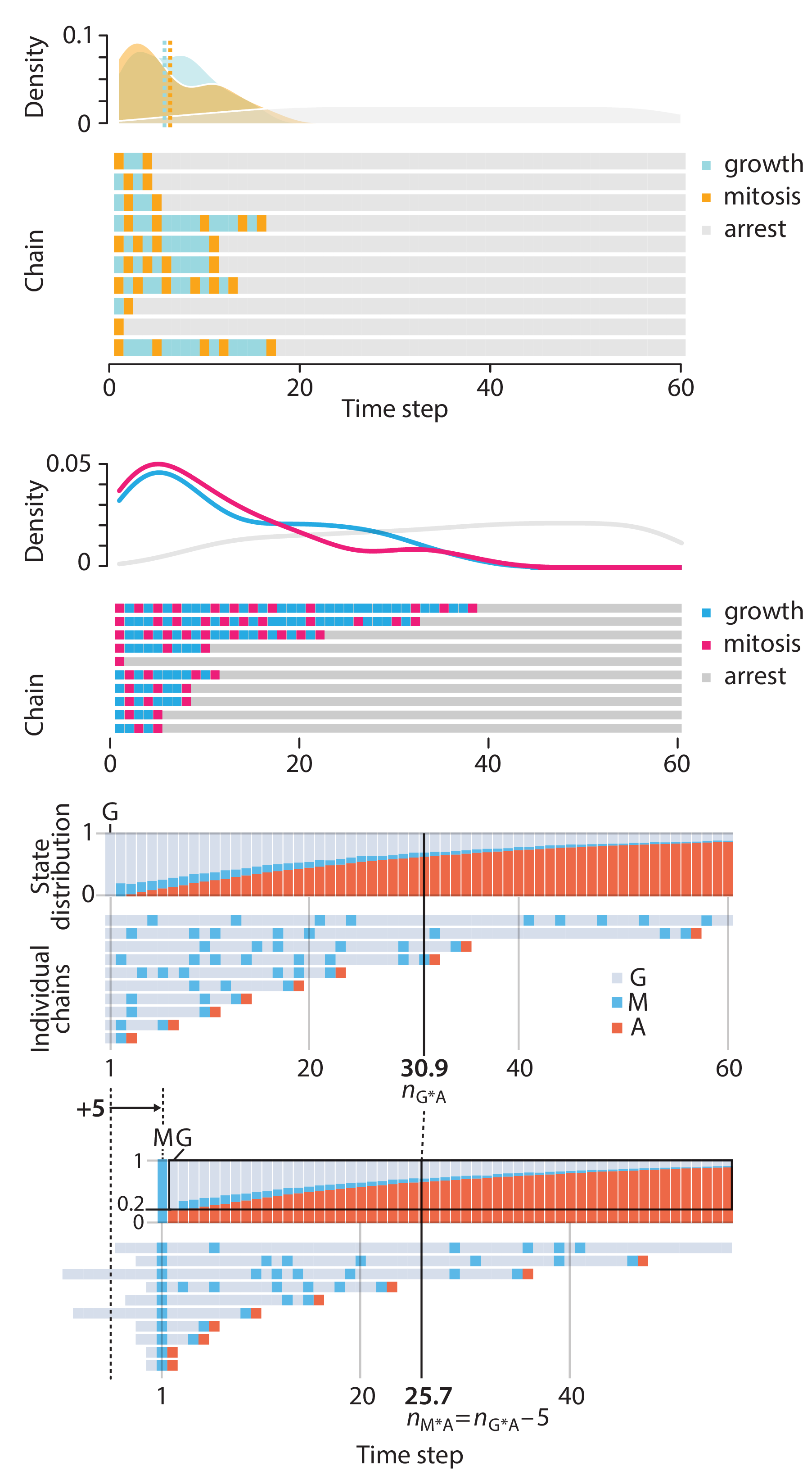
Altman, N. & Krzywinski, M. (2025) Crafting 10 Years of Statistics Explanations: Points of Significance. Annual Review of Statistics and Its Application 12:69–87.
Propensity score matching
I don’t have good luck in the match points. —Rafael Nadal, Spanish tennis player
In many experimental designs, we need to keep in mind the possibility of confounding variables, which may give rise to bias in the estimate of the treatment effect.
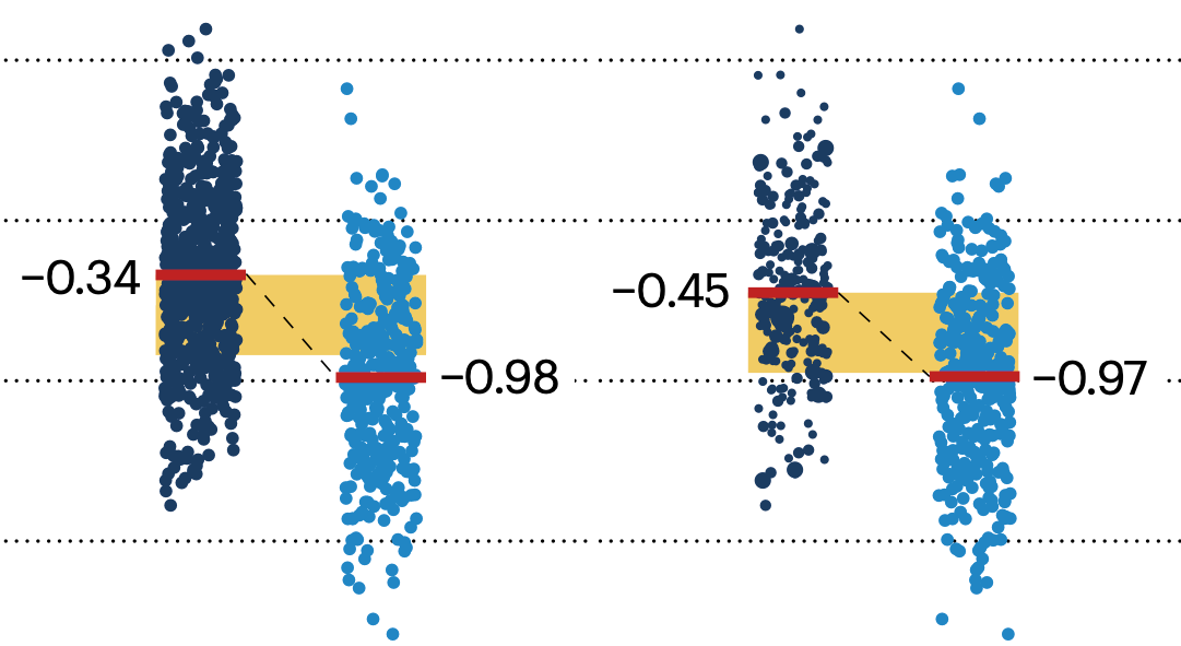
If the control and experimental groups aren't matched (or, roughly, similar enough), this bias can arise.
Sometimes this can be dealt with by randomizing, which on average can balance this effect out. When randomization is not possible, propensity score matching is an excellent strategy to match control and experimental groups.
Kurz, C.F., Krzywinski, M. & Altman, N. (2024) Points of significance: Propensity score matching. Nat. Methods 21:1770–1772.
Understanding p-values and significance
P-values combined with estimates of effect size are used to assess the importance of experimental results. However, their interpretation can be invalidated by selection bias when testing multiple hypotheses, fitting multiple models or even informally selecting results that seem interesting after observing the data.
We offer an introduction to principled uses of p-values (targeted at the non-specialist) and identify questionable practices to be avoided.
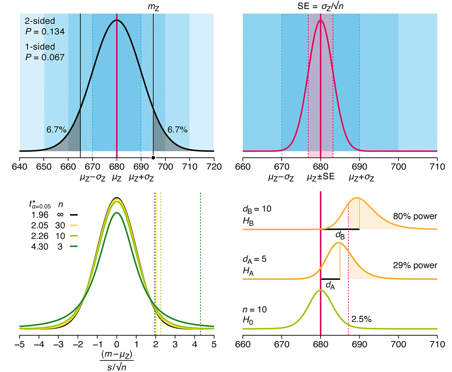
Altman, N. & Krzywinski, M. (2024) Understanding p-values and significance. Laboratory Animals 58:443–446.

