Color proportions in country flags
contents
Country flags are pretty colorful and some are even pretty.
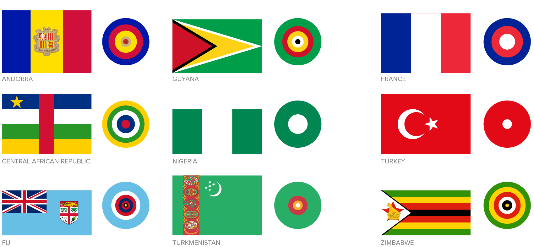
Instead of drawing the flag in a traditional way (yawn...), I wanted to draw it purely based on the color proportions in the flag (yay!). There are lots of ways to do this, such as stacked bars, but I decided to go with concentric circles. A few examples are shown below.
Once flags are drawn this way, they can be grouped by similarity in the color proportions.
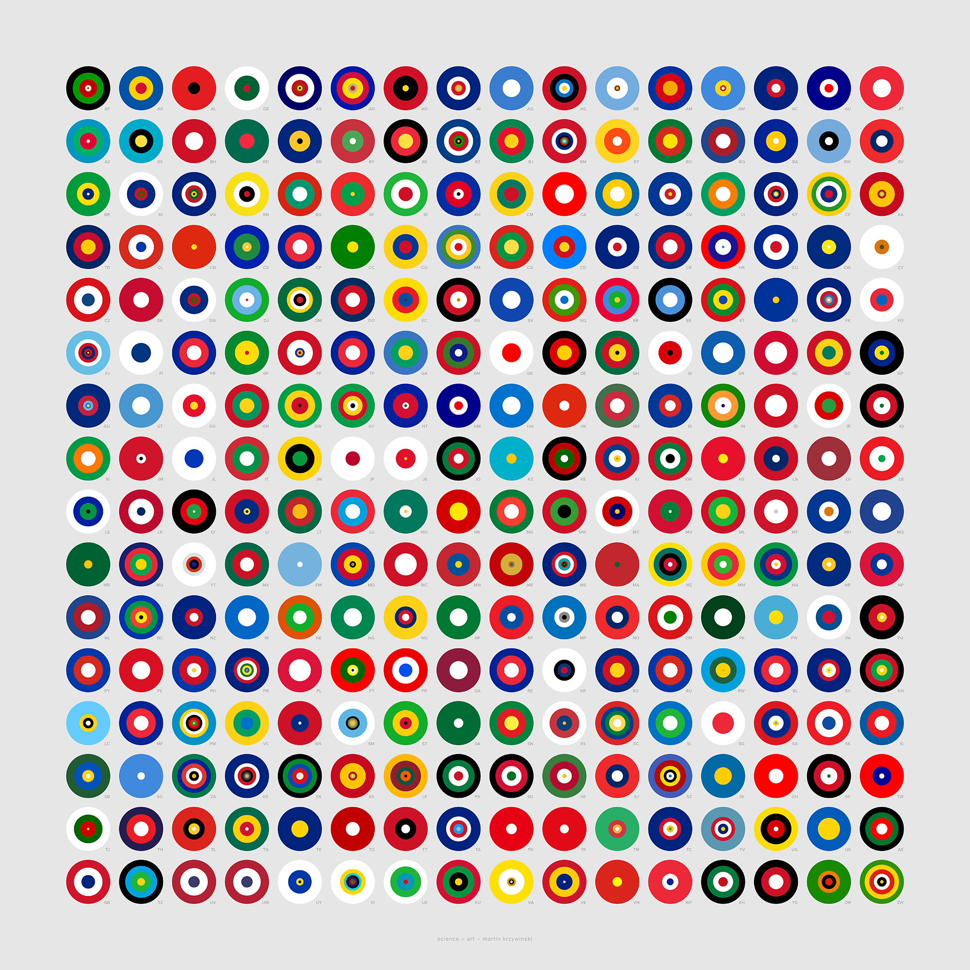
Check out the posters or read about the method below.
Or, download my country flag color catalog to run your own analysis.
To determine the proportions of colors in each flag, I started with the collection of all country flags in SVG from Wikipedia. The flags are conveniently named using the countries' ISO 3166-2 code. At the time of this project (21 Mar 2017), this repository contained 312 flags, of which I used 256.
I originally wanted to use the flag-icon-css collection, but ran into problems with it. It had flags in only either 1 × 1 or 4 × 3 aspect ratio, which distorted and clipped many flags. Many flags were also inaccurately drawn and had inconsistent use of colors. For example, in Turkey's flag the red inside the white crescent was slightly different than elsewhere in the flag.
 buy artwork
I converted the SVG files to high resolution PNG (2,560 pixels in width) and sampled the colors in each flag, keeping only those colors that occupied at least 0.01% of the flag. I apply this cutoff to avoid blends between colors due to anti-aliasing applied in the conversion. When drawing the flags as circles, I only use colors that occupy at least 1% of the flag—this impacts flags that have detailed emblems, such as Belize. I apply some rounding off of the proportions and colors with the same proportion are ordered so that lighter colors (by Lab luminance) are in the center of the circle.
There are various ways to represent the proportions of the flag colors as concentric rings—in other words, to use symbols of different size to encode area.
The accurate way is to have the area of the ring be proportional to the area of the color on the map. The inaccurate way is to encode the area by the the width of the ring. These two cases are the `k=0.5` and `k=1` columns in the figure below, where `k` is the power in `r = a^k` by which the radius of the ring, `r`, is scaled relative to the area, `a`. A perceptual mapping using `k=0.57` has been suggested by some.
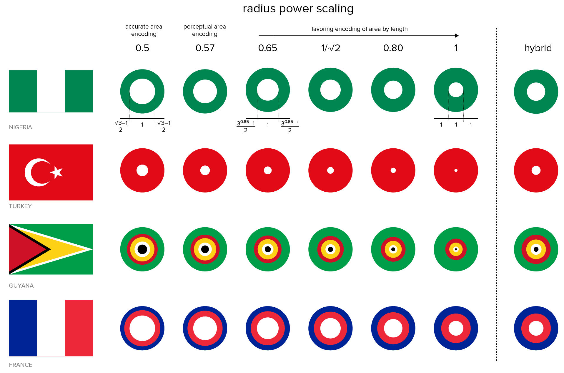
My goal here is not to encode the proportions so that they can be read off quantitatively. To find a value of `k`, I drew some flags and looked at their concentric ring representation. For example, with `k=0.57` the Nigerian flag's white center is too large for my eye while for `k=1` it is definitely too small. I liked the proportions for `k=1/\sqrt{2}` but wasn't happy with the fact that flags like France's, which have colors in equal areas, didn't have equal width rings.
In the end I decided on a hybrid approach in which the out radius of color `i` whose area is `a_i` is `r_i = a_i^k + \sum_{j=0}^{i-1} a_j^k` where the colors are sorted so that `a_{i-1} \le a_i`. If I use `k=0.25`, I manage to have flags like France have equal width rings but flags like Nigeria in which the proportions are not equal are closer to the encoding with `k=1/\sqrt{2}`. In this hybrid approach smaller areas, such as the white in the map of Turkey, are exaggerated. Notice that here `k` plays a slightly different role—it's used as the power for each color individually, `\sum a^k`, rather than their sum, `\left({\sum a}\right)^k`.
For the purists this choice of encoding might appear as the crime of the worst sort, representing neither correct (`k=0.5`) nor the conventionally incorrect encoding associated with `k=1`. Think of it this way—I know what rule I'm breaking.
The similarity between two flags is calculated by forming an intersection between the radii positions of the concentric rings of the flags.
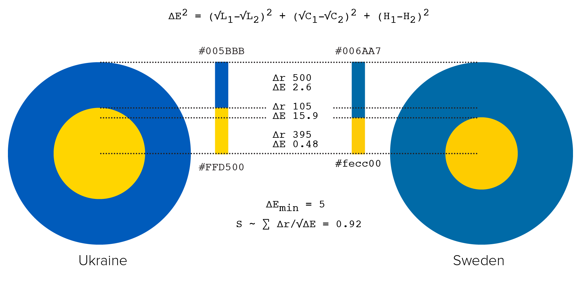
For each intersection, the similarity of colors is determined using `\Delta E`, which is the Euclidian distance of the colors in LCH space. I placed less emphasis on luminance and chroma in the similarity calculation by fist transforming the coordinates to `(\sqrt L,\sqrt C, H)`) before calculating color differences. The similarity score is $$ S = \sum \frac{\Delta r}{\sqrt{\Delta E}} $$
Color pairs with `\Delta E < \Delta E_{min} = 5` are considered the same and have an effective `\Delta E = 1`.
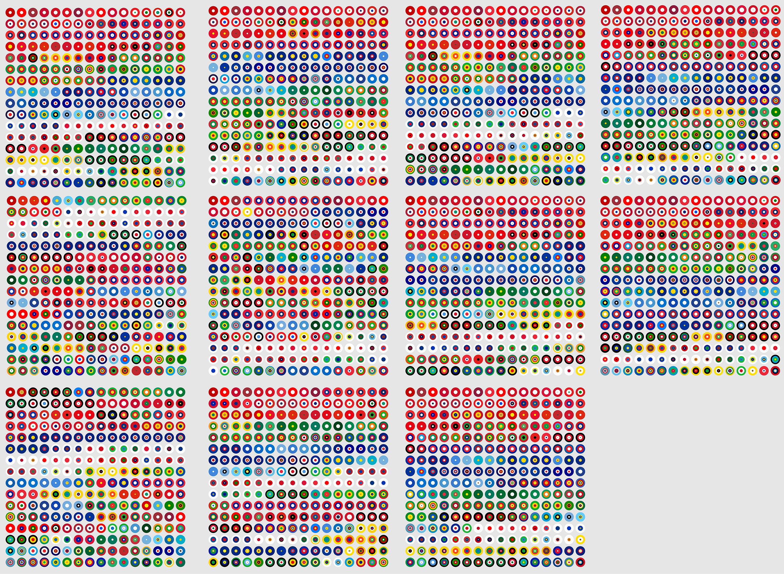
I explored different cutoffs and combinations of transforming the color coordinates. This process was informed based on how the order of the flags looked to me.
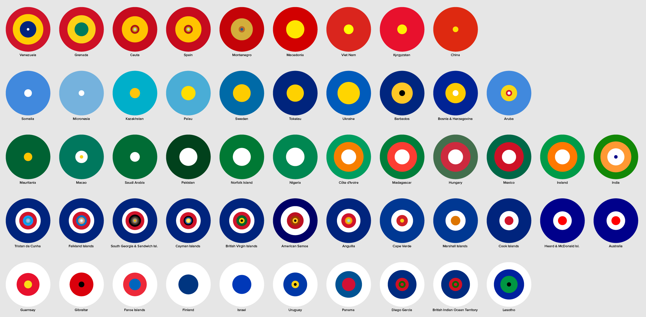
I decided to start the order with Tonga, since it had the highest average similarity score to all other flags in some of my trials. The flag that is most different from other flags, as measured by the average similarity score, is Israel.
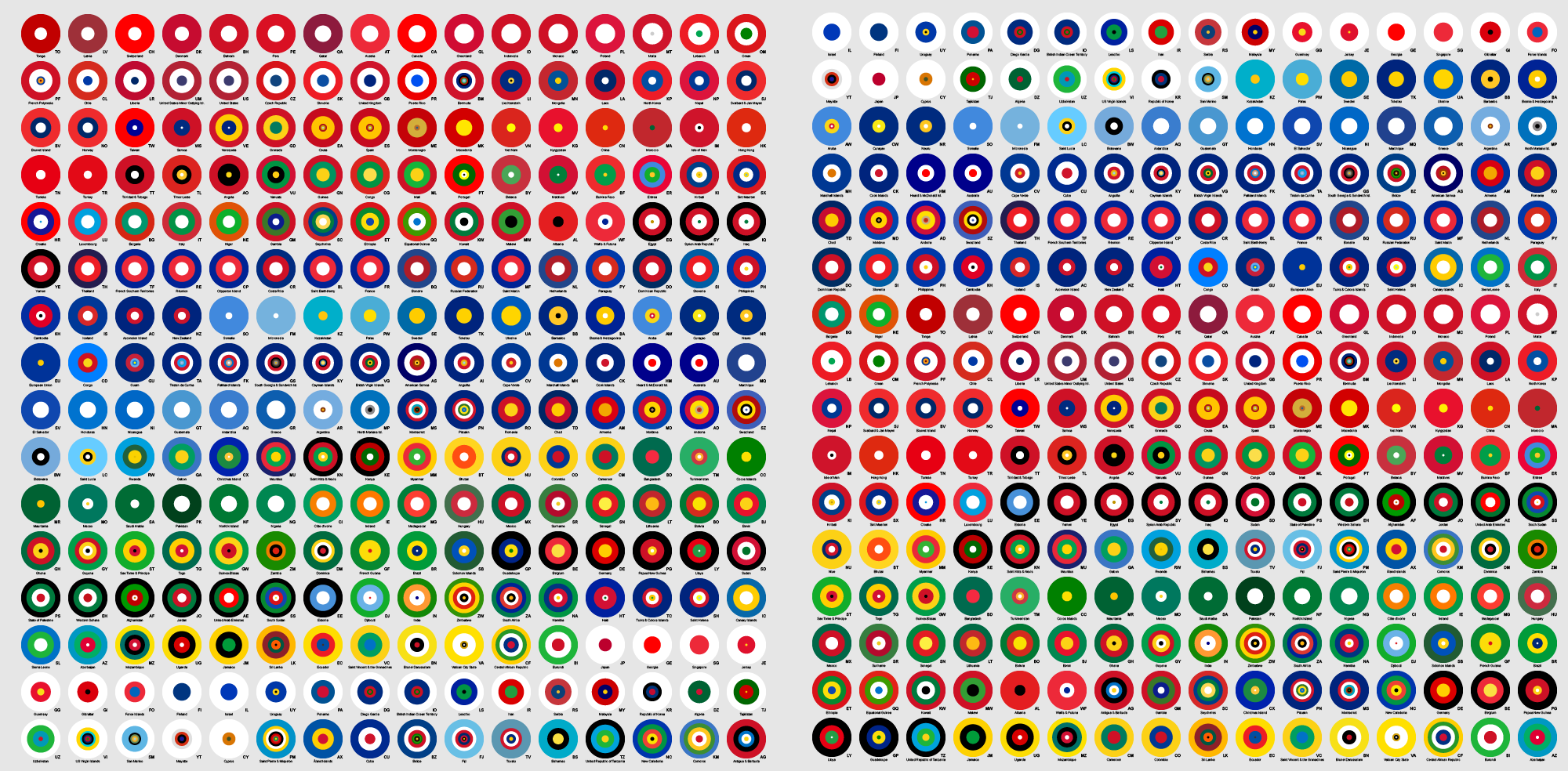
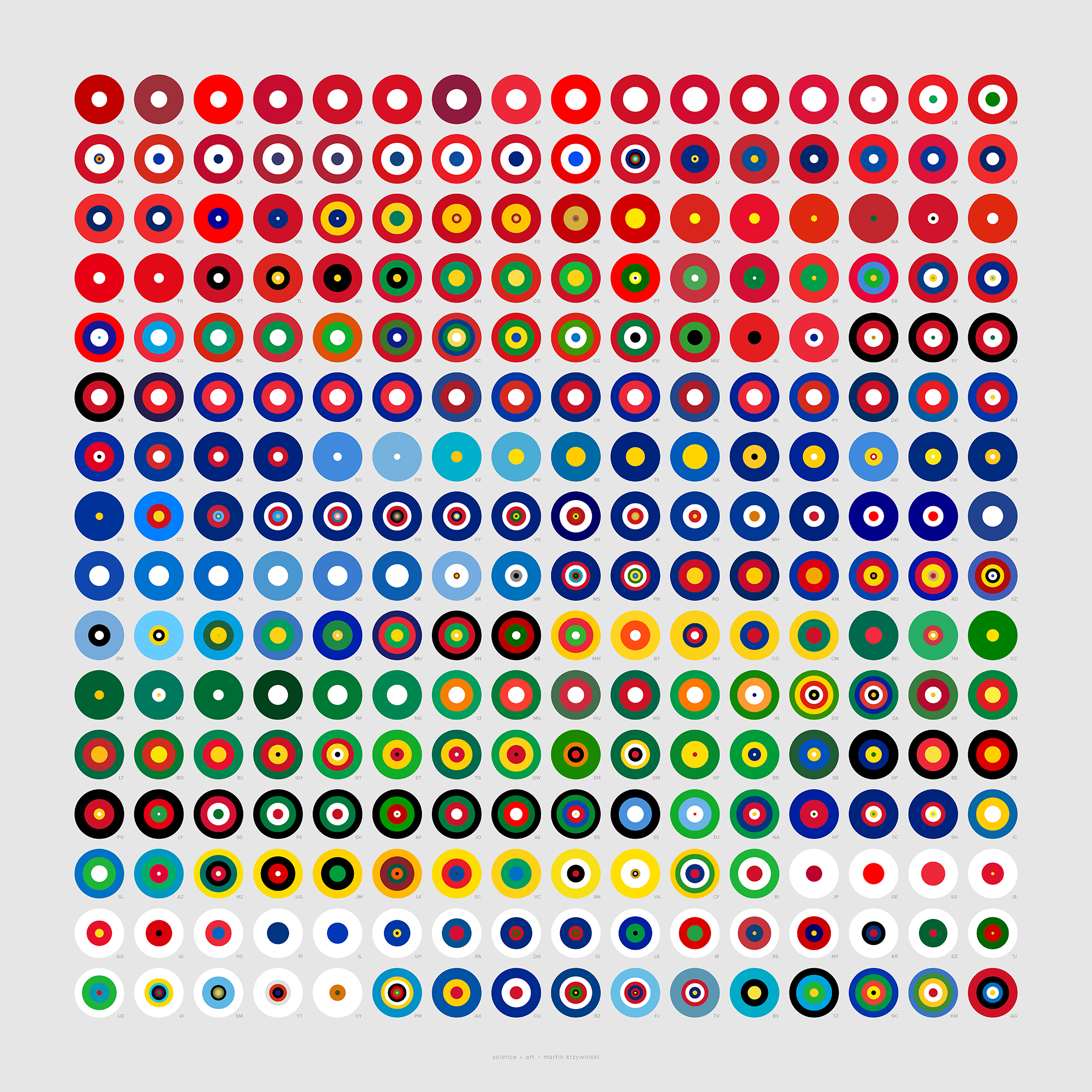 buy artwork
I couldn't find a list of colors in the flags of countries, so I provide my analysis here. Every country's SVG flag was converted into a 2,560 × 1,920 PNG file (4,915,200 pixels). Colors that occupied at least 0.01% of the pixels are listed in their HEX format, followed by the number of pixels they occupy. The fraction of the flag covered by sampled colors is also shown.
DOWNLOAD

#code img_pixels sampled_pixels fraction_sampled_pixels hex:pixels,hex:pixels,...
...
cm 4366506 4364514 0.999544 FCD116:1513103,007A5E:1456071,CE1126:1395340
cn 4369920 4364756 0.998818 DE2910:4260992,FFDE00:103764
co 4364800 4364800 1.000000 FCD116:2183680,003893:1090560,CE1126:1090560
...
DOWNLOAD

#code1 code2 similarity_score
ad ae 0.0108360578506763
ad af 0.0288161214840692
ad ag 0.0510922121861494
ad ai 0.42746294322472
...
zw ye 0.473278765746989
zw yt 0.238101673130705
zw za 0.810589244643825
zw zm 0.573265751850587
Beyond Belief Campaign BRCA Art
Fuelled by philanthropy, findings into the workings of BRCA1 and BRCA2 genes have led to groundbreaking research and lifesaving innovations to care for families facing cancer.
This set of 100 one-of-a-kind prints explore the structure of these genes. Each artwork is unique — if you put them all together, you get the full sequence of the BRCA1 and BRCA2 proteins.
Propensity score weighting
The needs of the many outweigh the needs of the few. —Mr. Spock (Star Trek II)
This month, we explore a related and powerful technique to address bias: propensity score weighting (PSW), which applies weights to each subject instead of matching (or discarding) them.
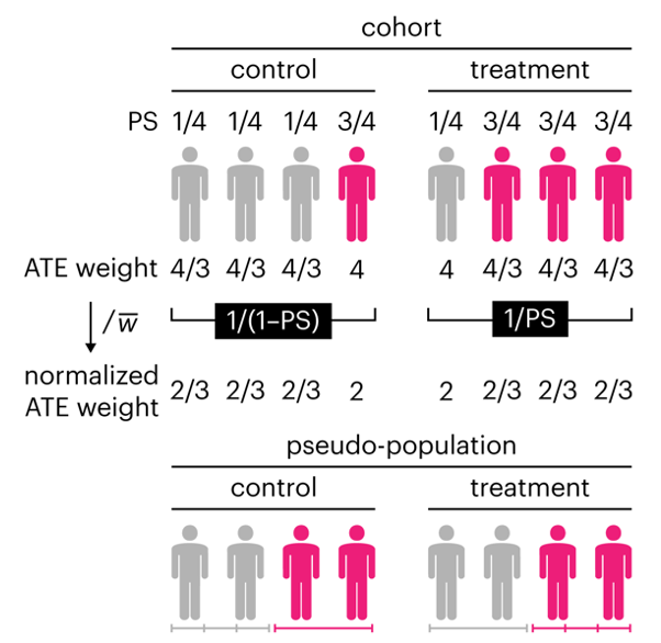
Kurz, C.F., Krzywinski, M. & Altman, N. (2025) Points of significance: Propensity score weighting. Nat. Methods 22:1–3.
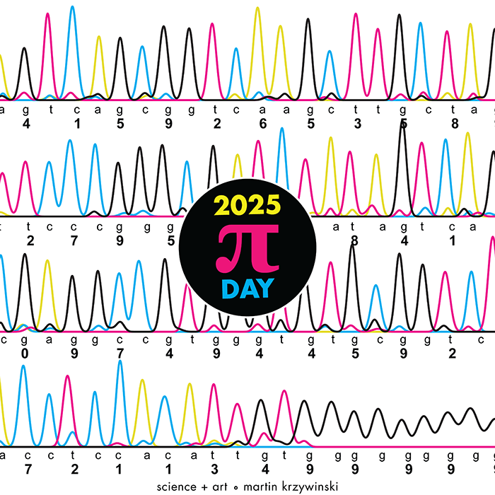
Happy 2025 π Day—
TTCAGT: a sequence of digits
Celebrate π Day (March 14th) and sequence digits like its 1999. Let's call some peaks.
Crafting 10 Years of Statistics Explanations: Points of Significance
I don’t have good luck in the match points. —Rafael Nadal, Spanish tennis player
Points of Significance is an ongoing series of short articles about statistics in Nature Methods that started in 2013. Its aim is to provide clear explanations of essential concepts in statistics for a nonspecialist audience. The articles favor heuristic explanations and make extensive use of simulated examples and graphical explanations, while maintaining mathematical rigor.
Topics range from basic, but often misunderstood, such as uncertainty and P-values, to relatively advanced, but often neglected, such as the error-in-variables problem and the curse of dimensionality. More recent articles have focused on timely topics such as modeling of epidemics, machine learning, and neural networks.
In this article, we discuss the evolution of topics and details behind some of the story arcs, our approach to crafting statistical explanations and narratives, and our use of figures and numerical simulations as props for building understanding.
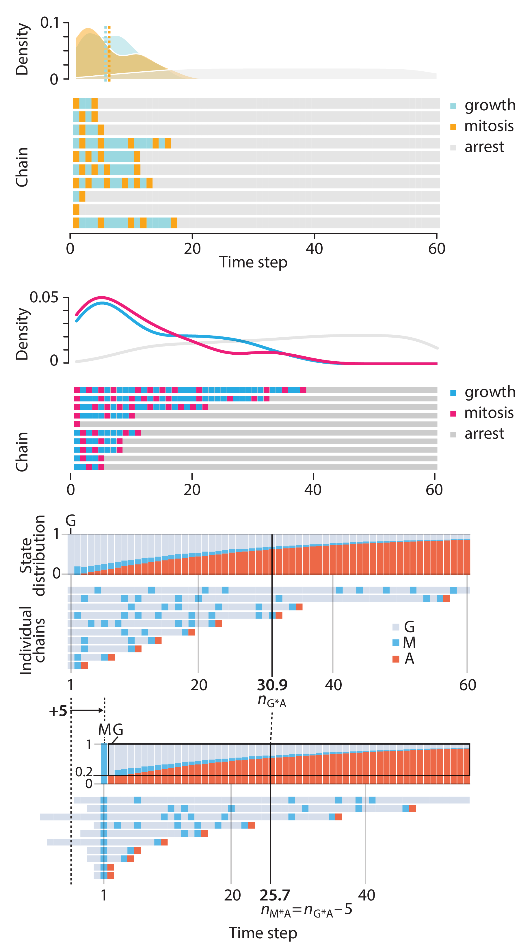
Altman, N. & Krzywinski, M. (2025) Crafting 10 Years of Statistics Explanations: Points of Significance. Annual Review of Statistics and Its Application 12:69–87.
Propensity score matching
I don’t have good luck in the match points. —Rafael Nadal, Spanish tennis player
In many experimental designs, we need to keep in mind the possibility of confounding variables, which may give rise to bias in the estimate of the treatment effect.
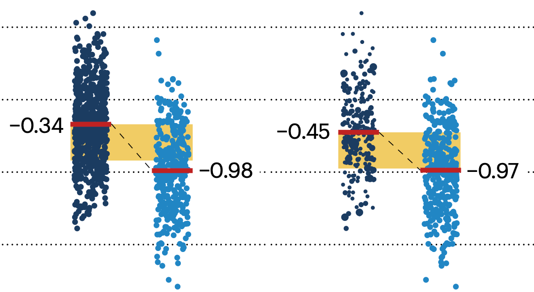
If the control and experimental groups aren't matched (or, roughly, similar enough), this bias can arise.
Sometimes this can be dealt with by randomizing, which on average can balance this effect out. When randomization is not possible, propensity score matching is an excellent strategy to match control and experimental groups.
Kurz, C.F., Krzywinski, M. & Altman, N. (2024) Points of significance: Propensity score matching. Nat. Methods 21:1770–1772.
Understanding p-values and significance
P-values combined with estimates of effect size are used to assess the importance of experimental results. However, their interpretation can be invalidated by selection bias when testing multiple hypotheses, fitting multiple models or even informally selecting results that seem interesting after observing the data.
We offer an introduction to principled uses of p-values (targeted at the non-specialist) and identify questionable practices to be avoided.
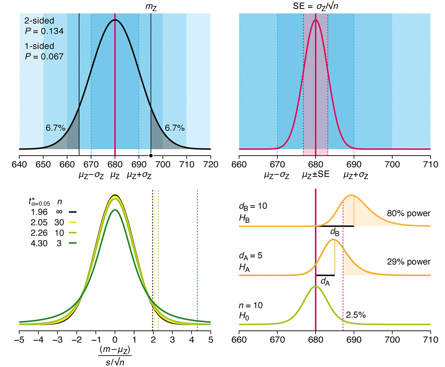
Altman, N. & Krzywinski, M. (2024) Understanding p-values and significance. Laboratory Animals 58:443–446.
