Tarred by the same brush as other scripting languages, Perl (which in fact is semi-compiled), is perceived as too slow and memory-devouring for heavy numerical computations because it doesn't lend itself to storing and retrieving zillions of numbers quickly. This has been a source of great frustration to the authors, both enthusiastic Perl (ab)users who resent being forced to use more primitive environments for their astronomical data analysis. Perl's potential for manipulating numerical data sets speedily and elegantly via an extension was obvious. Hence PDL, the Perl Data Language, was born. PDL is a Perl extension, so you get the convenience of programming in Perl with the speed of compiled C.
PDL introduces a new data structure: the "pdl numerical array," often referred to as a "piddle." (This unfortunate nickname has led to some rather dubious puns in the source code.) Anyway, a piddle is a special object that can contain a large block of efficiently-stored numbers for manipulation with normal mathematical expressions. For example, if $a is a piddle containing a 3x4x6 chunk of data, then the Perl statement $b = sin($a) will do exactly what you think: set $b equal to $a but with every value replaced its sine. Easy - and because each operation is implemented via compiled C code, it's nearly as fast as a hand-crafted C program.
Complete Listing of PDL Functions (as of PDL 1.11).
PDL can be used "normally" from a script - simply use PDL. But it also has a shell interface for interactive data analysis and prototyping. Here we'll play with the PDL shell, called perldl, which we'll invoke from the command line.( This article assumes you have PDL-1.11, PGPLOT-2.0 (which itself requires the pgplot graphics library), and Perl 5.003. If you also have the right versions of the Term::ReadLine and Term::ReadKey modules, the perldl shell allows interactive command line editing.)
% perldl

perlDL shell v1.11

Loaded PDL v1.11   ReadLines enabled


Reading /home/frossie/.perldlrc ...

	          perldl>
The perldl shell behaves like Perl's debugger. For instance, we can assign values to variables and print them with p:
perldl> $b = 2

perldl> p $b/2

1

perldl> p $b/3

	0.666666666666667

perldl>
Since PDL is really about matrices, let's create a 2x3 matrix and multiply it by itself:
perldl> $a = pdl [5,3,4], [6,4,3];

perldl> print $a;

[

  [5 3 4]

  [6 4 3]

]

perldl> $b = $a * $a;

perldl> print $b;

[

  [25 9 16]

  [36 16 9]

]
But to have true fun with PDL, we'll first need some data. Luckily the PDL distribution comes with a picture of the sky stored in FITS, the standard format for astronomical data. PDL also supplies rfits(), a function that reads FITS files and returns a piddle containing the data. So let's read in our image and plot it:
perldl> $a = rfits "PDL1.11/m51.fits";

IO loaded

BITPIX = 16 size = 65536 pixels

Reading  131072 bytes

BSCALE = 1.0000000000E0 && BZERO = 0.0000000000E0


perldl>
Now we have data - and we didn't have to spend three nights freezing up a mountain to get it. What do we know about it? That it is 16-bit with 65536 elements. But is it 65536x1 or 256x256 or even 16x16x16x16?
perldl> p dims $a

256 256

perldl>
Not surprisingly (after all, it's a picture of the sky) we have a two-dimensional image: 256x256. dims() is a PDL function that returns the dimensions of a piddle. But what about the data values?
perldl> p stats $a

104.193572998047 67.4254211880158

perldl>
So there - stats() is a PDL function than returns the mean and standard deviation of a piddle. We can even print some of it now-Jon might get upset if we displayed 65536 numbers, so let's go for the bottom left corner instead:
perldl> p sec($a,0,3,252,255)

[

 [50 51 54 53]

 [50 50 53 54]

 [51 52 53 52]

 [54 53 54 51]

]


perldl>
sec() returns a section of a piddle; the above statement displays the rectangle between elements (0,252) and (3,255). Additional dimensions are handled seamlessly: just pass the extra coordinate values as arguments.
Perhaps you're getting restless at this point. Let's abandon the function calls and jump to the cool stuff.
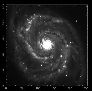
perldl> imag $a

Loaded PGPLOT

Displaying 256 x 256 image from 24 to 500 ...
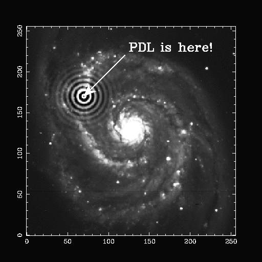
which pops up a window displaying this figure:
My god Dave, it's full of stars! And so it should be - this is in fact an image of Messier 51, a spiral galaxy similar to our own but at a distance of 200,000,000,000,000,000,000 miles away, give or take a few billion. That's a bit too far for us to invade, but we can at least humiliate it:
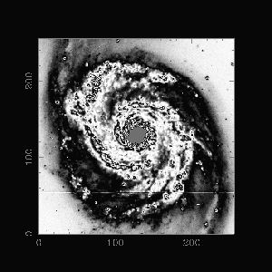
perldl> imag sin(0.05*$a)

Displaying 256 x 256 image from -0.999990224838257 to 0.999992072582245 ...
Since we're exploring cosmology, let's create something out of nothing:
perldl> $r = rvals zeroes 20,20
As you can see, PDL functions can be chained together just like Perl functions. Two PDL functions are cascaded here: rvals() and zeroes(). First, zeroes() creates a piddle full of zeroes-in this case, a 20x20 matrix with every element zero. (There's also a ones() function.)
Then rvals() fills that piddle with values representing the distance of each element from the center.
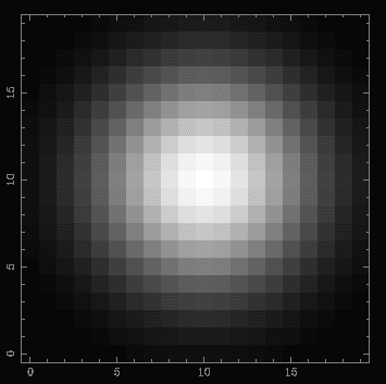
perldl> $g = exp(-($r/6)**2)/108.08

perldl> imag $g
...which displays the following:
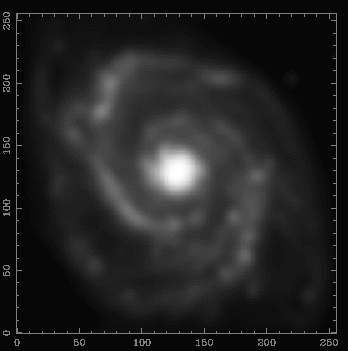
Alert readers (assuming there are any left at this point) will note that the exp() function was used to generate a two-dimensional Gaussian. The less mathematically inclined will say it looks like a blob. Let's inflict a bit more punishment on Messier 51 by convolving it with our newly-created Gaussian filter. This enables us to simulate what we would see if we were observing through very bad viewing conditions, such as a (possibly drunken) haze.
perldl> $b = convolve $a,$g

perldl> imag $b
You might want to know that this operation takes 20-25 seconds on a Pentium 120 or Sparc 20 with PDL. Doing this with a 2D array in normal (non-PDL) Perl takes 13 minutes and uses 11 times as much memory. Is that cool or what?
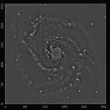
perldl> imag $a-$b
Ah, an unsharp masked image! This is often used in astronomy to emphasize sharp features against a bright background, such as stars in a galaxy, the giant luminous gas clouds we call HII ("aitch-two") regions, or foreground objects such as UFO's (err, weather balloons).
So that's how it all works.
Where are we now?
PDL was prototyped early in 1996 and is currently in beta release. (One author's habit of prototyping Perl modules while on astronomical observing trips leaves the other author wondering whether this is a previously unknown symptom of altitude sickness.) It is functional but not yet fully featured. It is under vigorous development thanks to the work and enthusiasm of the perldl mailing list participants. The current stable version is 1.11.
Several auxiliary modules for PDL are nearing completion: 3D graphic manipulation using OpenGL (Tuomas J. Lukka), an interface to the Meschach matrix library (Etienne Grossmann), an interface to the XMGR plotting tool (Tim Jenness), access to the TIFF, GIF, PostScript, and other formats supported by PBM+ (Christian Soeller), and an interface to the SLATEC numerical library (Tuomas J. Lukka). Other formats are under development for PDL 2.0, which will also feature virtual slicing, easier C extensions, and fast implicit looping.
Anyone wishing to reflect or opine on the rather technical issues surrounding PDL development is welcome to join the perldl mailing list at perldl-request@jach.hawaii.edu or the porters list at pdl-porters-request@jach.hawaii.edu. Send your questions to the former and your complaints to the latter. Finally, the obligatory URL: https://www.aao.gov.au/local/www/kgb/perldl/, which includes Christian Soeller's PDL FAQ.
Stay tuned...
Karl Glazebrook is an astronomer at the Anglo-Australian Observatory, and Frossie Economou is a software engineer and astronomer at the UK Infrared Telescope in Hawaii.
