Infinity with Max Cooper — In Six Minutes
Great fleas have little fleas upon their backs to bite ’em,
And little fleas have lesser fleas, and so ad infinitum.
And the great fleas themselves, in turn, have greater fleas to go on;
While these again have greater still, and greater still, and so on.
—Augustus de Morgan
contents
- 1 · Oh my God, it's full of numbers
- 2 · One, two, three, infinity
- 3 · Glitches in the story
- 4 · Hilbert's Grand Hotel
- 5 · New bijections await
- 6 · Last stop before switching infinity trains
- 7 · Beyond infinity — other infinities
- 8 · Power set of natural numbers
- 9 · Cardinality of the continuum
- 10 · Aleph 2
The video starts straight at number 1 and go to infinity (and beyond). Let's go!
The walkthrough includes key mathematical details behind the theory of transfinite numbers. The story is aimed at a math-enthusiast audience. For even more details for the hardy and curious, I cover some advanced concepts in set theory, such as beth numbers and ordinal numbers.
This math may cause you to lose sleep. I hope it does, as many things in life are worth staying awake for.
Take care — I'm not a set theoretician. Please report errors, technical shortcomings and places where you feel the explanations are lacking.
The video begins humbly is with the first natural number, 1.
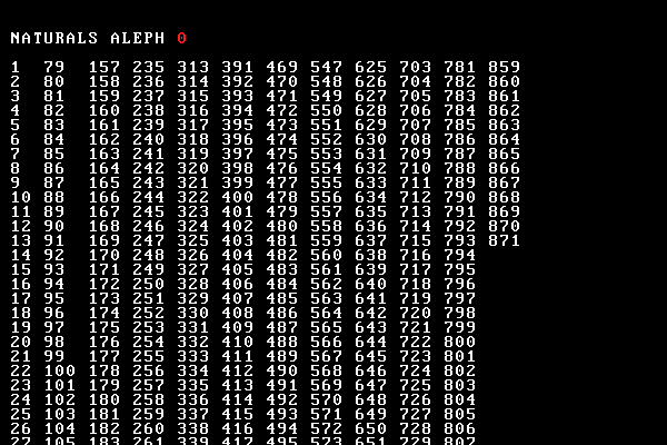
What follows are all the other natural numbers—everyone has their favourite. I like 17.
All the natural numbers make up a set, $\mathbb{N}$. $$\mathbb{N} = \{ 1, 2, 3...\}$$
We never run out of these numbers—to get the next one just take the previous and add one. This process of adding one to get the next number is called the successor function. For now, this is easy but we'll see below an application of this that's a little trickier.
How big is $\mathbb{N}$? In set theory, the size of a set is referred to as its cardinality and denoted by $|\mathbb{N}|$. At this point you might simply want to answer "It's infinitely large!" and be done with it.
Hang around, though. This is just where the story gets interesting.
To acknowledge the fact that your mind might glitch while investigating infinity, you'll see that the music video glitches as well.
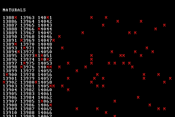
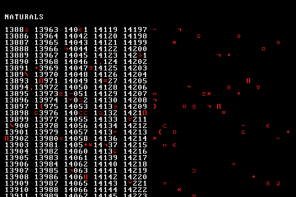
As the video progresses, the frequency and intensity of the glitching is increased and new set theory symbols are added. Many of the glitches are triggered by the snare drum. As the percussion becomes more intense, so does the glitching.
The video ends with a return to the counting of natural numbers which then glitches into a blank screen and only `\aleph` remains.
There is a magical place called the Grand Hotel. It has an infinite number of rooms, each indexed by a natural number.

Despite the fact that this hotel is always completely full, it can always accommodate another guest. To do this, we ask everyone to move to room $n+1$ thus freeing up room $1$. We have solved the problem at the cost of annoying infinitely many people.
But wait. There's infinitely more.
The hotel can always accommodate an additional infinite number of guests. Everyone is asked to move to room $2n$ thus freeing up all odd-numbered rooms. Since there's an infinite number of these rooms, we've just doubled the capacity!
I don't mean to suggest that I loved you the best
I can't keep track of each fallen robin
I remember you well in the Chelsea Hotel
That's all, I don't even think of you that often
— Leonard Cohen, Chelsea Hotel No. 2
The craziness is only beginning. If an infinite number of busses show up, each with an infinite number of guests, guess what? Yup, they can all be accommodated.
First, denote the $i$th guest in the $j$th bus by $s_n = (i,j)$. Since $i \in \mathbb{N}$ and $j \in \mathbb{N}$ then, we can enumerate $s_n$ as $s_1, s_2, s_3, ...$ Then, the formula for assigning guests to rooms is to assign guest $i$ from bus $j$ to room $n$. In this scheme, the hotel itself is treated as a bus indexed by $j = 0$.
This is sometimes called “Hilbert's Paradox” but it's not really a paradox. Rather, it's a demonstration that we should not expect intuition about finite quantities to carry over to the behaviour of infinite quantities.
Case in point, in Hilbert's hotel "there is a guest in every room" does not imply that "no more guests can be accommodated".
Your mind may be in revolt at this moment. “Surely, there are fewer even numbers than natural numbers, since even numbers are a proper subset of natural numbers!”
First, in a hotel with finite number of rooms, you would be correct.
Second, your confusion puts you in good company. Gregor Cantor (1845-1918), the mathematician who was the first to develop a theoretical framework of infinite quantities, suffered recurrent nervous breakdowns.
Remember the concept of the cardinality of a set? Cantor assigned the number $\aleph_0$ (named so after the first letter, aleph, in the Hebrew alphabet) to represent the cardinality of the naturals.
He called the family of numbers, in which $\aleph_0$ is the first, transfinite numbers . Today ‘infinite’ is more commonly used to refer to these numbers.
For two sets to have the same cardinality a special condition has to be met. We say that $|X| = |Y|$ if and only if we can demonstrate a function $f(X) \mapsto Y$ that is one-to-one, meaning that $f(x \in X)$ maps to a unique $y \in Y$, and onto, meaning that every $y \in Y$ is mapped to by some $x \in X$.
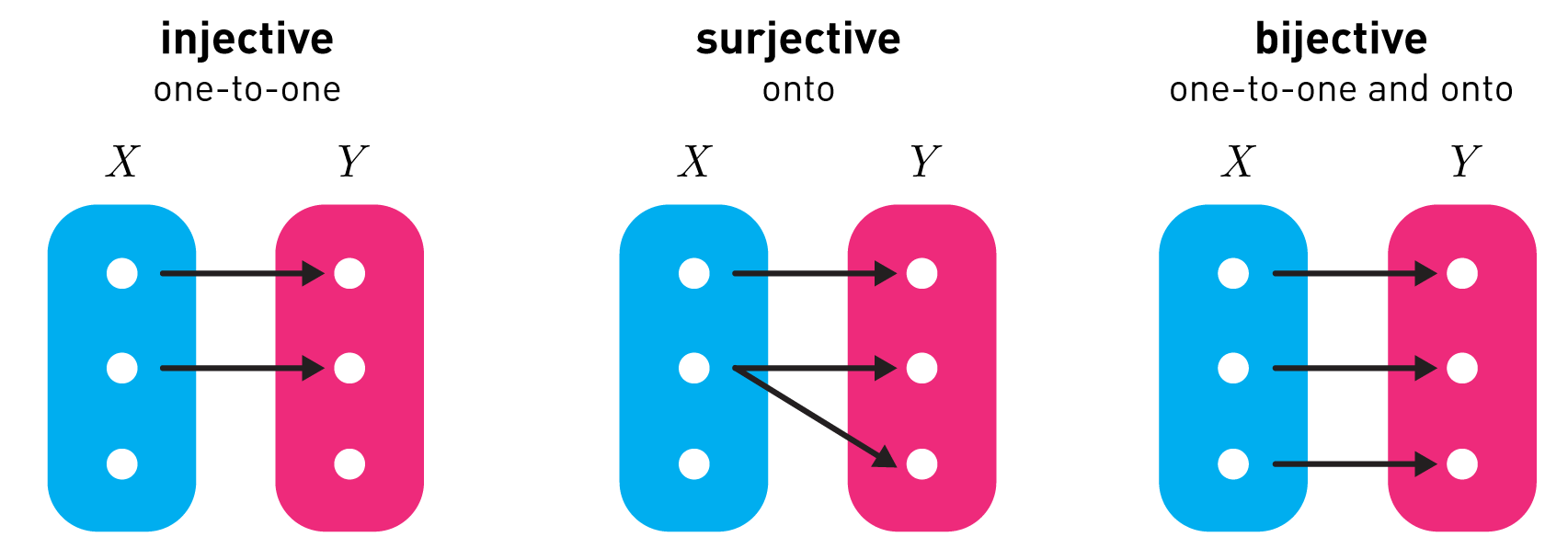
In other words, to show that two sets have the same cardinality, we just have to find a bijection. Here is one between the even numbers and natural numbers $$ f(\{2,4,6,8,...\} \mapsto \mathbb{N}) : x \mapsto x/2 $$
To show that $f$ is a bijection we need to show that $f$ is injective and surjective. It is injective (one-to-one) since any two distinct even numbers $x \ne y$ are sent to distinct values $x/2 \ne y/2$. It is surjective (onto) since every natural number $x$ has an even number $2x$ that is mapped to it.
There are lots of sets that have the same cardinality as the naturals: odd numbers, even numbers, prime numbers. Any infinite subset of naturals has the same cardinality as the naturals.
The next chapter in the video brings us to the observation that since the naturals are a subset of the integers, $\mathbb{Z}$ and since both are infinite, both have to have the same cardinality.
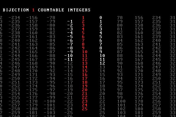
The video shows a bijection between the two sets, $f(\mathbb{N}) \mapsto \mathbb{Z}$ defined as follows: $f(0) \mapsto 0$ and $f(2k) \mapsto k$, $f(2k-1) \mapsto -k$ for $k \in \mathbb{N}$. Even naturals are sent to positive integers and odd naturals are sent to negative integers. Each natural has a unique integers (injective) and all integers are covered (surjective).
For example, the positive integer $n$ is mapped from $2n \in \mathbb{N}$ (e.g. $22 \mapsto 11$) and the negative integer $-n$ from $-(2n-1)$ (e.g. $23 \mapsto -11$).
The next part of the video shows many more possible bijections.
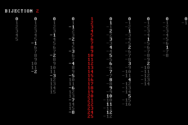
The first column on the right of the naturals is the bijection described above and others take the form $$f(x \in \mathbb{N}) = \begin{cases} 0, & \text{if $x = 1$} \\k, & \text{if $x$ is the $k$th number that passes the rule $g(x)$} \\-k, & \text{if $n$ is the $k$th number that fails the rule $g(x)$} \end{cases} $$
For our first bijection, the rule was $g(x) \stackrel{?}{=} 2k$, which checks whether $x$ is even.
The second column on the right of the naturals uses the rule $g(x) \stackrel{?}{=} 4k$, which checks whether $x$ is a multiple of 4. Thus, $4 \mapsto 1$, $8 \mapsto 2$, $12 \mapsto 3$ and so on. All naturals that are not multiples of 4 are sent to negative integers.
Columns on the left of the naturals use an odd multipler in the $g(x)$ rule and additionally flip the sign of the integer to which $f(x)$ maps. This was done so that I could have an equal balance of white positive integers in the columns on the right and white negative integers in the columns on the left.
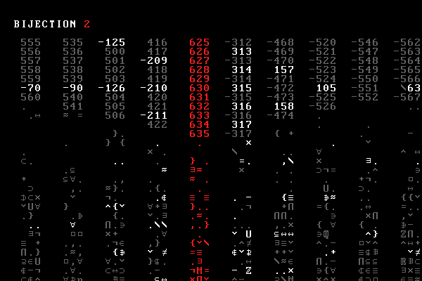
As we sample more natural numbers, pages of bijections update faster and faster, in waves of numbers that decay into symbols used in set theory.
Because I could not stop for Death —
He kindly stopped for me —
The Carriage held but just Ourselves —
And Immortality.
...
Since then — 'tis Centuries — and yet
Feels shorter than the Day
I first surmised the Horses' Heads
Were toward Eternity —
— Emily Dickinson
We ramp up the complexity in the video by showing a bijection between the natural numbers and rational numbers, $\mathbb{Q}$, which are all fractions of the form $\mathbb{Q} = \{ q = x/y, x,y \in \mathbb{N}_0, y \ne 0 \}$.
First, we create a table in which the cell in row $x$ and column $y$ is assigned the rational number $x/y$.
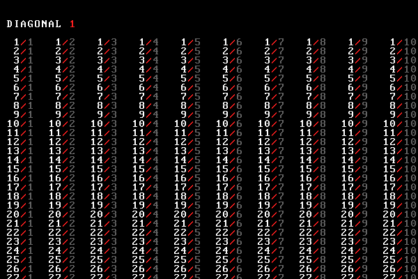
To create the bijection, we assign each rational to a natural number as we traverse the table in a zig-zag fashion.
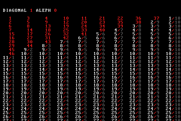
We snake our way from the upper-left corner ($1/1$) to the bottom-right ($78/31$), which is assigned 2418.
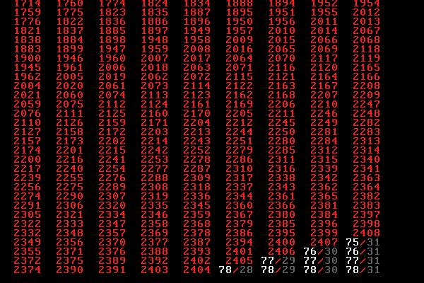
Given that rational numbers can be considered as two-dimensional naturals, $\mathbb{Q} = \mathbb{N}^2 = { \mathbb{N} \times \mathbb{N} }$, the same traversal argument can be used to show that all higher-dimensional spaces of naturals also have the same cardinality as the naturals, $|\mathbb{N}^k| = |\mathbb{N}|$. The bijection construction is the same as in the $k=2$ case above, except that now we're snaking across a higher dimensional space. When $k$ itself is infinite, we have the scenario of infinite guests in infinite busses arriving at Hilbert's Grand Hotel.
In our story so far, we have shown bijections between $\mathbb{N}$ and $\mathbb{Z}$ and $\mathbb{Q}$ we have proven that all these sets have the same cardinality $|\mathbb{N}| = |\mathbb{Z}| = |\mathbb{Q}| = \aleph_0$.
To summarize, the naturals are considered to be infinite but countable and any set that has a bijection with the naturals is also countable.
Our discussion has brought us to infinity, $\aleph_0$. What lies beyond?
The first hint that there is indeed something beyond lies in the proof that the real numbers, $\mathbb{R}$ are not countable: there is no bijection between the naturals and reals. If we try to pair up naturals and reals we'll always run out of naturals.
Real numbers are continuous quantities that, for example, can measure the distance along a line. They include the naturals, integers, rationals as well as irrationals, which include numbers like $\sqrt{2}$, which cannot be written as a fraction, and numbers like $\pi$, which are transcendentals and not solutions to polynomial equations.
Cantor's demonstration that $|\mathbb{R}| > |\mathbb{N}|$ is the next part of the story. The proof is by contradiction and applies to the unit interval $ [0,1) = \{ x \, | \, 0 \le x \lt 1 \}$. First, suppose that there is a bijection $f(\mathbb{N}) \mapsto [0,1)$. This implies that for each $n \in \mathbb{N}$ there is some associated $r \in [0,1)$. We write down this assignment—for each natural, we pair up a natural with a real from the unit interval. Obviously, this list goes on forever in both the vertical and horizontal direction.
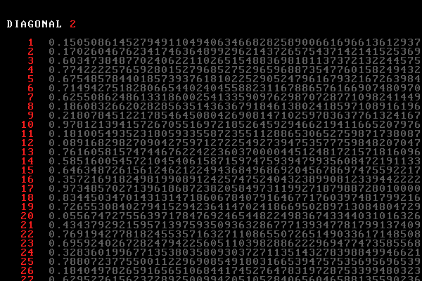
We don't know what the exact assignment is, so the numbers in the story are only representative. Typically, the proof is written out symbolically with each natural $n_i$ assigned to a series of digits $n_{i1}n_{i2}n_{i3} ... $.
Because this assignment is a bijection it is a surjection and every real number from the unit interval appears somewhere in the list. If we could demonstrate that there is a real number from $[0,1)$ that doesn't appear in the list, we would have a contradiction and the assumption that a bijection exists would be invalid.
We do so as follows. We transform the first digit of the first real to $x \mapsto x + 1 \, \text{mod} \, 10$. In other words $0 \mapsto 1$, $1 \mapsto 2$ and $9 \mapsto 0$.
We do the same for the second digit of the second number, the third digit of the third number, and so on.
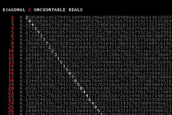
This creates a new real, shown here without the leading $0.$
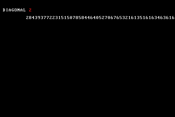
By construction, this real is nowhere in our list of reals. It can't be—it's different from each of the reals in at least one digit. It's different from the first number in the first digit, the second number in the second digit, the third number in the third digit and so on. But it's obviously in the unit interval. A contradiction.
If we write the numbers in the unit interval in binary $ [0,1) = \{ 0.b_1b_2b_3,... \, | \, b \in \{0,1\} \}$ we can use the fact that $b_i$ is indexed by $\mathbb{N}$ to realize that there are $2^{|\mathbb{N}|}$ such binary numbers, since at each position we have two choices ($0$ or $1$). And because $|\mathbb{N}| = \aleph_0$ we have $$ |\mathbb{R}| = 2^{|\mathbb{N}|} = 2^{\aleph_0} $$
Given a set $X$, the power set is the set of all subsets of $X$, including the empty set.
The next part of the story builds up the power set of naturals, $\mathbb{P}(\mathbb{N})$.
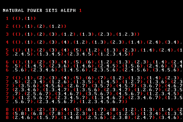
For example, for $X = \{1\}$ the power set has two elements, the empty set $\{\}$ and the whole set $\{1\}$. We write $ \mathbb{P}(X) = \{\{\},\{1\}\} $.
For $X = \{1,2\}$ the power set has four elements, the empty set $\{\}$, each of the naturals on their own $\{1\}$ and $\{2\}$ and the whole set $\{1,2\}$. We write $ \mathbb{P}(X) = \{\{\},\{1\},\{2\},\{1,2\}\} $.
In general, the power set of $\{1,2,3,...,n\}$ has cardinality $2^n$.
If we look closely at the $ 2^{\aleph_0} $, we can interpret it as the cardinality of the power set of naturals. This is because for each natural, of which there are $ \aleph_0 $ we have two choices: put it in the subset or not.
As the video continues, the power set elements appear faster and faster. The braces form hypnotising patterns.
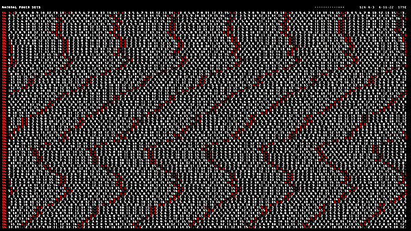
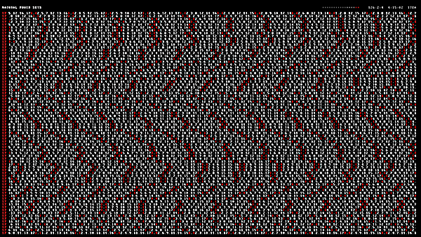
Because the reals are continuous quantities, the number of reals is (wonderfully) called the cardinality of the continuum. I wouldn't turn down the job of cardinal of the continuum.
Given what we learned about power sets of naturals above, we can write $$ |\mathbb{R}| = | \mathbb{P}(\mathbb{N}) | = 2^{\aleph_0} $$
With Cantor's diagonal proof, we know that $|\mathbb{R}| > \aleph_0$ but we don't know how much larger. Cantor therefore proposed the Continuum Hypothesis which stated that whatever the size of $2^{\aleph_0}$ was, it was a distinct kind of infinite number and, importantly, the next smallest infinite number after $\aleph_0$.
A consequence of this theorem is that there is no set $X$ for which $$ \aleph_0 \lt |X| \lt 2^{\aleph_0} $$
meaning that there is no set that is larger than the naturals but smaller than the reals.
The Continuum Hypothesis also implies that the cardinality of the continuum is the next number ($\aleph_1$) in the hierarchy of transfinite cardinals, $$ |\mathbb{R}| = 2^{\aleph_0} = \aleph_1 $$
From it, we also get that the cardinality of the power set of an infinite set is the next transfinite cardinal. In other words, for sets $\mathbb{N}, \mathbb{P}(\mathbb{N}), \mathbb{P}(\mathbb{P}(\mathbb{N})), ...$ the cardinalities are $\aleph_0, \aleph_1, \aleph_2, ...$ And in general, $$ \aleph_{\alpha+1} = 2^{\aleph_\alpha} $$
The Continuum Hypothesis is thus far unproven.
At this point, we arrive at the third infinity in the video—the cardinality of the power set of reals is $ | \mathbb{P}({\mathbb{R}}) | = \aleph_2 $.
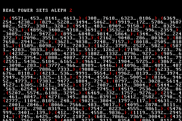
Elements of the power sets of naturals and reals continue to flash. If the Continuum Hypothesis is true, their cardinality is $\aleph_1$ and $\aleph_2$ respectively.
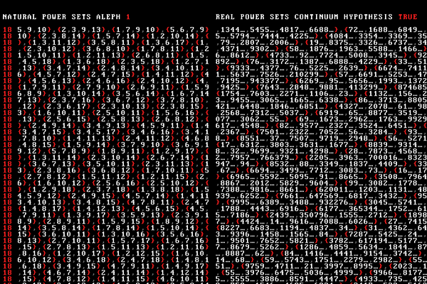
The music grows in intensity and the scene deteriorates into set theory symbols.
The story brings us back to where we started from: the list of naturals. These pick up where we left off and continue counting.
These too decay in a jitter of symbols
with soon nothing but symbols left
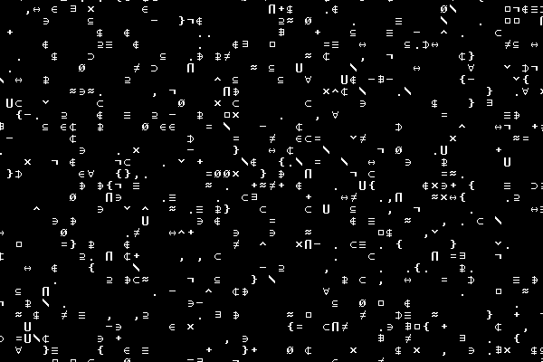
Suddently $\aleph$ appears.
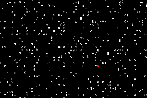
And while everything else decays,
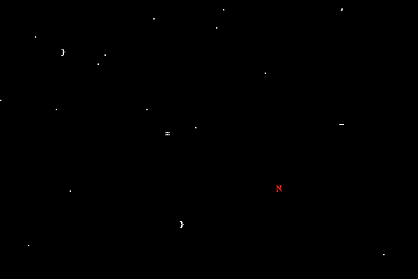

We are reminded of where we started, how far we've gone and how many more infinites are left to go.
How many ages hence
Shall this our lofty scene be acted over,
In states unborn and accents yet unknown!
— William Shakespeare
And so, in our yearning for the infinite, we return to basic counting and find that we never understood it well in the first place.
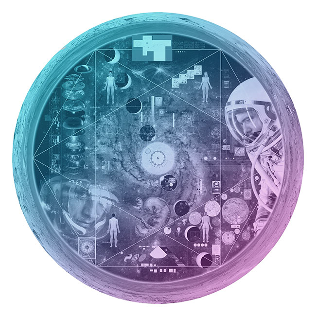
Nasa to send our human genome discs to the Moon
We'd like to say a ‘cosmic hello’: mathematics, culture, palaeontology, art and science, and ... human genomes.


Comparing classifier performance with baselines
All animals are equal, but some animals are more equal than others. —George Orwell
This month, we will illustrate the importance of establishing a baseline performance level.
Baselines are typically generated independently for each dataset using very simple models. Their role is to set the minimum level of acceptable performance and help with comparing relative improvements in performance of other models.
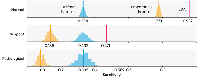
Unfortunately, baselines are often overlooked and, in the presence of a class imbalance5, must be established with care.
Megahed, F.M, Chen, Y-J., Jones-Farmer, A., Rigdon, S.E., Krzywinski, M. & Altman, N. (2024) Points of significance: Comparing classifier performance with baselines. Nat. Methods 20.
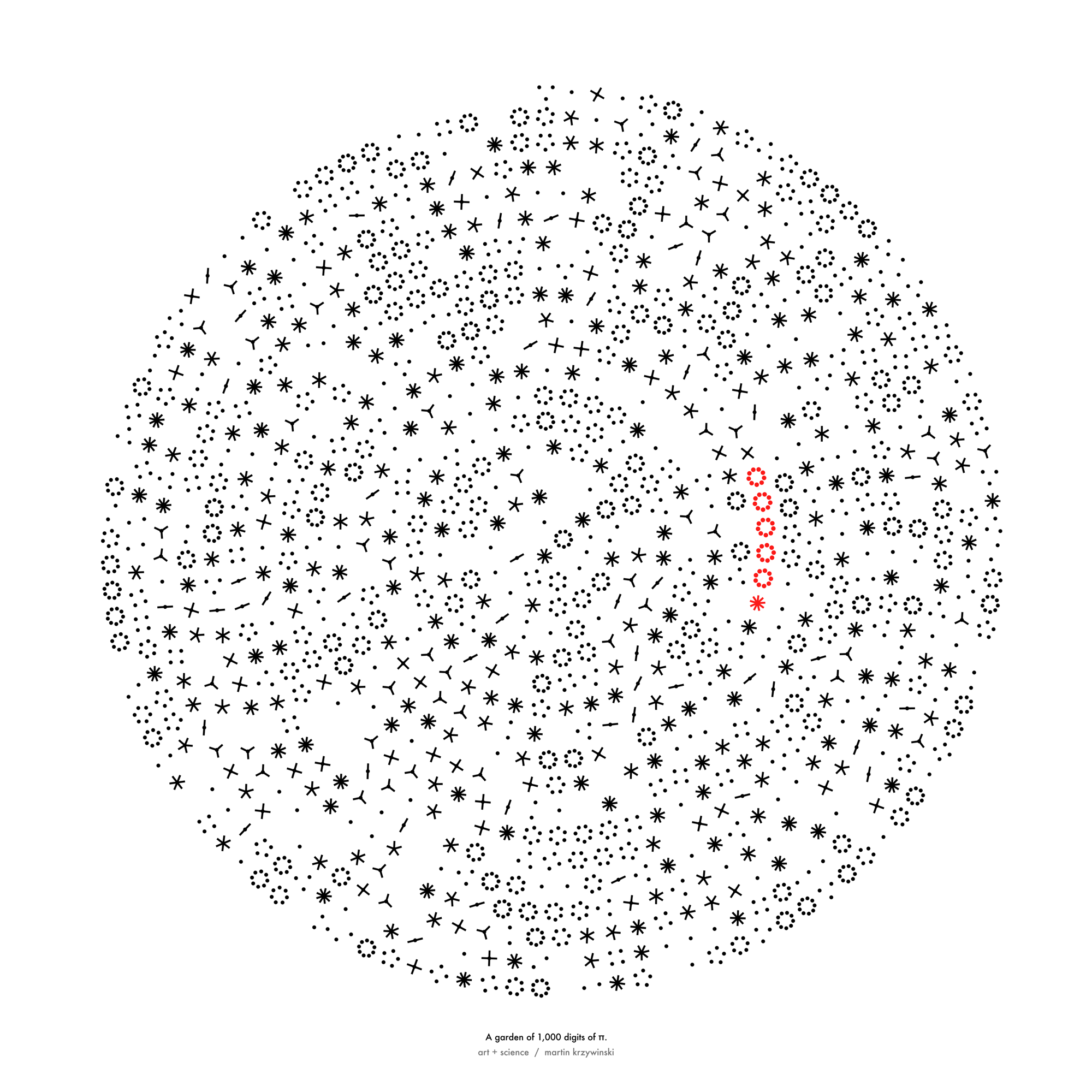
Happy 2024 π Day—
sunflowers ho!
Celebrate π Day (March 14th) and dig into the digit garden. Let's grow something.
How Analyzing Cosmic Nothing Might Explain Everything
Huge empty areas of the universe called voids could help solve the greatest mysteries in the cosmos.
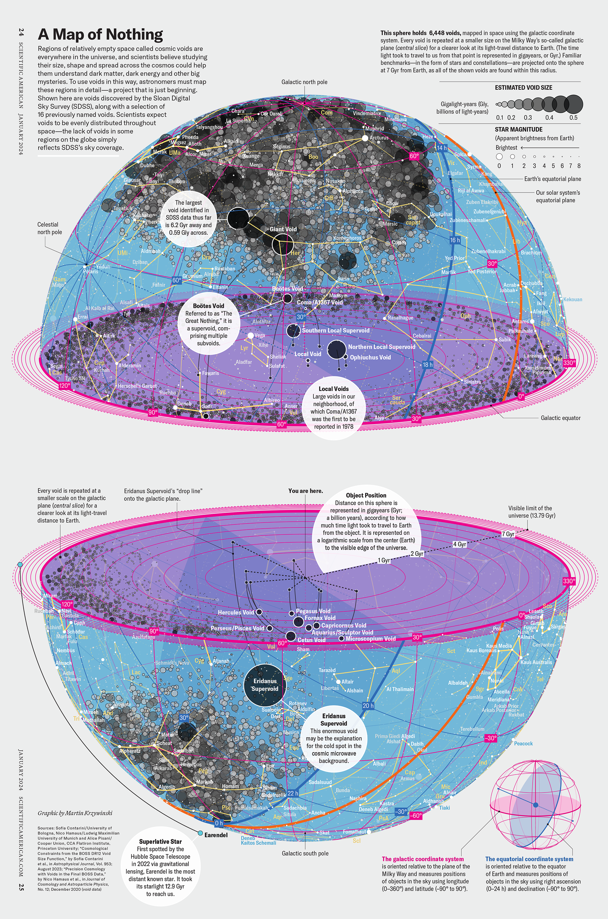
My graphic accompanying How Analyzing Cosmic Nothing Might Explain Everything in the January 2024 issue of Scientific American depicts the entire Universe in a two-page spread — full of nothing.
The graphic uses the latest data from SDSS 12 and is an update to my Superclusters and Voids poster.
Michael Lemonick (editor) explains on the graphic:
“Regions of relatively empty space called cosmic voids are everywhere in the universe, and scientists believe studying their size, shape and spread across the cosmos could help them understand dark matter, dark energy and other big mysteries.
To use voids in this way, astronomers must map these regions in detail—a project that is just beginning.
Shown here are voids discovered by the Sloan Digital Sky Survey (SDSS), along with a selection of 16 previously named voids. Scientists expect voids to be evenly distributed throughout space—the lack of voids in some regions on the globe simply reflects SDSS’s sky coverage.”
voids
Sofia Contarini, Alice Pisani, Nico Hamaus, Federico Marulli Lauro Moscardini & Marco Baldi (2023) Cosmological Constraints from the BOSS DR12 Void Size Function Astrophysical Journal 953:46.
Nico Hamaus, Alice Pisani, Jin-Ah Choi, Guilhem Lavaux, Benjamin D. Wandelt & Jochen Weller (2020) Journal of Cosmology and Astroparticle Physics 2020:023.
Sloan Digital Sky Survey Data Release 12
Alan MacRobert (Sky & Telescope), Paulina Rowicka/Martin Krzywinski (revisions & Microscopium)
Hoffleit & Warren Jr. (1991) The Bright Star Catalog, 5th Revised Edition (Preliminary Version).
H0 = 67.4 km/(Mpc·s), Ωm = 0.315, Ωv = 0.685. Planck collaboration Planck 2018 results. VI. Cosmological parameters (2018).
constellation figures
stars
cosmology
Error in predictor variables
It is the mark of an educated mind to rest satisfied with the degree of precision that the nature of the subject admits and not to seek exactness where only an approximation is possible. —Aristotle
In regression, the predictors are (typically) assumed to have known values that are measured without error.
Practically, however, predictors are often measured with error. This has a profound (but predictable) effect on the estimates of relationships among variables – the so-called “error in variables” problem.
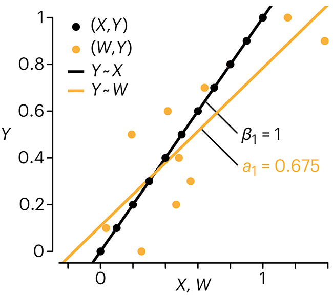
Error in measuring the predictors is often ignored. In this column, we discuss when ignoring this error is harmless and when it can lead to large bias that can leads us to miss important effects.
Altman, N. & Krzywinski, M. (2024) Points of significance: Error in predictor variables. Nat. Methods 20.
Background reading
Altman, N. & Krzywinski, M. (2015) Points of significance: Simple linear regression. Nat. Methods 12:999–1000.
Lever, J., Krzywinski, M. & Altman, N. (2016) Points of significance: Logistic regression. Nat. Methods 13:541–542 (2016).
Das, K., Krzywinski, M. & Altman, N. (2019) Points of significance: Quantile regression. Nat. Methods 16:451–452.
Convolutional neural networks
Nature uses only the longest threads to weave her patterns, so that each small piece of her fabric reveals the organization of the entire tapestry. – Richard Feynman
Following up on our Neural network primer column, this month we explore a different kind of network architecture: a convolutional network.
The convolutional network replaces the hidden layer of a fully connected network (FCN) with one or more filters (a kind of neuron that looks at the input within a narrow window).
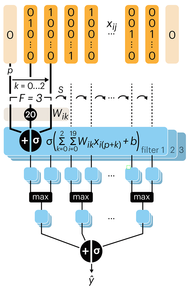
Even through convolutional networks have far fewer neurons that an FCN, they can perform substantially better for certain kinds of problems, such as sequence motif detection.
Derry, A., Krzywinski, M & Altman, N. (2023) Points of significance: Convolutional neural networks. Nature Methods 20:1269–1270.
Background reading
Derry, A., Krzywinski, M. & Altman, N. (2023) Points of significance: Neural network primer. Nature Methods 20:165–167.
Lever, J., Krzywinski, M. & Altman, N. (2016) Points of significance: Logistic regression. Nature Methods 13:541–542.


