Infinity with Max Cooper — In Six Minutes
Only I discern—
Infinite passion, and the pain
Of finite hearts that yearn.
—Robert Browning
contents
If you've studied transfinite numbers before, you'll no doubt notice that some core ideas have been left out from the video, such as ordinals and Beth numbers.
The math behind these adds a layer of complexity to the story that we felt was unnecessary for a first and dynamic telling of the ideas. They're explained below, for those who are hardy to follow this deep.
We already saw that the cardinality of the naturals defined the first transfinite number $ | \mathbb{N} | = \aleph_0$. If the continuum hypothesis holds, the cardinality of the power set of the naturals and the cardinality of the continuum was the next in the $\aleph$ hierarchy, $ | \mathbb{P}(\mathbb{N}) | = | \mathbb{R} | = \aleph_1$.
The story is a little more complicated than this.
The size of power sets is expressed by a family of transfinite cardinals called $ \beth $ (Beth) numbers. I think that the $\beth$ numbers are easier to understand.
The cardinality of the naturals is defined as $|\mathbb{N}| = \beth_0$ and the cardinality of their power set is the next $\beth$, $|\mathbb{P}(\mathbb{N})| = \beth_1$. Taking the power set again, $|\mathbb{P}(\mathbb{P}(\mathbb{N}))| = \beth_2$, $|\mathbb{P}(\mathbb{P}(\mathbb{P}(\mathbb{N})))| = \beth_3$, and so on.
In general, a set of cardinality $\beth_\alpha$ the cardinality of its power set is $\beth_{\alpha+1}$. In other words, $$ \beth_{\alpha+1} = 2^{\beth_\alpha} $$
As we saw, the cardinality of the continuum is the same as the cardinality of the power set of naturals, $ | \mathbb{R} | = | \mathbb{P}(\mathbb{N}) | = \beth_1$. Using the definition above for stepping up the $\beth$ hierarchy, the cardinality of the power set of the continuum is $ | \mathbb{P}(\mathbb{R}) | = \beth_2 $, $ | \mathbb{P}(\mathbb{P}(\mathbb{R})) | = \beth_3 $, and so on.
By definition, $\aleph_0 = \beth_0$.
Also by definition, there are no infinite cardinalities between $\aleph_0$ and $\aleph_1$. And since infinite cardinalities are linearly ordered (we can compare their sizes) it means that $$ \aleph_1 \le \beth_1 $$
and in general $$ \aleph_\alpha \le \beth_\alpha $$
If the Continuum Hypothesis is true, then $$ \aleph_1 = \beth_1 $$
There may be transfinite numbers indexed by $\aleph$ that are not indexed by $\beth$. For example, if the Continuum Hypothesis is false, then it's possible that $\beth_1 > \aleph_1$ and so $\aleph_1$ doesn't appear in the set of $\beth$ numbers.
You may have noticed that while the definition of $\aleph_1$ was relatively brief. We said that it is the cardinality of the continuum if the Continuum Hypothesis holds.
In actual fact, $\aleph_1$ has a specific definition that arises from another family of numbers—the ordinals.
$\aleph_1$ is defined as the cardinality of the countable ordinal numbers. To understand this, we have to look at ordinal numbers and how they differ from cardinal numbers.
Cardinals, which express the size of a set, can be used to classify sets based on their cardinality. A set of three apples and a set of three bananas have the same cardinal classification because they have the same size.
Orderinals express the rank or order of something. For example, the ordinal 42 is intrepreted as 42nd and implies that 41 things came before it (if we started at $1$). The cardinal 42 has no such implication—you can have 42 bananas in a bag and there is no expectation that there ever was a bag with 41 bananas.
The rank of the biggest loser in a race is an ordinal (they came in 42nd) but the total size of the field is cardinal (there were 42 racers in total).
Although most of the numbers we use are cardinals, the distinction between cardinals and ordinals is practically irrelevant for finite quantities. Thus, the examples above (bananas and racres) are almost painfully trivial. The subtle distinctions between cardinals and ordinals in the context of finite quantities belie the deep differences between them in general.
Mathematically, ordinals classify sets based on their well-order. In order to unpack this, we have to understand a little bit about how set order is defined.
We first define something called a total order, which is a function that can be used to establish an order for elements in a set. For example, $\le$ is one such total order and $\gt$ is another. This function applies to a pair of elements and identifies which one comes first.
A set with a total order is a totally ordered set. This is nothing more than some set (e.g. the naturals) and some total order (e.g. $\le$).
Now, such a totally ordered set is said to be well-ordered if every non-empty subset of the set has a least element. This is the part that's very important and it's here that the first sign of confusion may arise. In particular, even though it doesn't look like much, the statement “has a least element” is very powerful.
Consider the set of naturals, $\mathbb{N}$. This set is well-ordered using the total order $\le$. This is because every subset of the naturals has a least element, as defined by $\le$.
However, the integers are not well-ordered under $\le$ because we can find a subset of them (e.g. negative integers) that don't have a least element. This is because for any member in the set of negative integers, $-n$ there is always a smaller one, $-n-1$.
This doesn't meant that the integers can't be well-ordered—they can, we just have to pick a different total order. For example, one function under which the integers are well-ordered places them in the order $0,1,2,3,...,-1,-2,-3,...$. Under this function, $3$ comes before $-1$. Keep in mind that the use of the word ‘least’ in this context implies ‘first’ not ‘smallest’ because we're talking about order and not size.
The reals are not well ordered under the $\lt$ operation since any open subset doesn't have a least element. For example, the interval $(0,1)$ doesn't have a least element since for any small number $0 < \epsilon$ there is a smaller number $ 0 < \epsilon' < \epsilon$. However, the reals can be put into a well-order, as described by the Well-ordering Theorem that states that every set can be well-ordered.
A lucid definition of ordinals is provided by von Neumann: the von Neumann ordinals.
He defined the first ordinal trivially as the empty set, $\varnothing$. He then defined the next ordinal as the set that includes all the previous ordinals, $\{\varnothing\}$. Don't confuse the difference between $x$ and $\{x\}$. The former is the object $x$ and the latter is the set that contains the object $x$. These two are as different as a banana and a bag that contains a banana.
According to this rule, the third ordinal would be the set of the first two ordinals, $\{ \varnothing, \{\varnothing\} \}$.
Here are the first 5 ordinals in this definition $$ \begin{array}{cll} 0 & \{ \} & \varnothing \\1 & \{ 0 \} & \{\varnothing\} \\2 & \{ 0,1 \} & \{\varnothing,\{\varnothing\}\} \\3 & \{ 0,1,2 \} & \{ \varnothing, \{\varnothing\}, \{ \varnothing, \{ \varnothing \} \} \} \\4 & \{ 0,1,2,3 \} & \{ \varnothing, \{\varnothing\}, \{\varnothing,\{\varnothing\}\}, \{ \varnothing, \{\varnothing\}, \{ \varnothing, \{ \varnothing \} \} \} \} \\\end{array} $$
The labels $0, 1, 2, ...$ in the table above are a visual aid to shorten the notation and better communicate the relationship between the structures in the right-most column. Do not think of these labels as ‘numbers’ and certainly not as cardinal numbers.
When written this way, ordinal numbers are sets. Moreover, every member of every ordinal number is a subset. For example, the ordinal $2 = \{0,1\}$ is a member of $3$ but it's also a subset of $3$ because both $0$ and $1$ are members of $3$. Here I have used the labels in the table above to stand in for the set definitions of each of the ordinals.
The ordering of the ordinals is defined by set membership (containment). The ordinals are thus well-ordered.
Given an ordinal, $\alpha$, we can create the next ordinal by $\{ \alpha, \{ \alpha \} \}$. This rule is called a successor function, $$ S(\alpha) = \{ \alpha, \{ \alpha \} \} $$
and in the table above, we've simply applied the successor function iteratively to $\varnothing$. To see this more clearly, consider the ordinal $\{0,1\}$. Applying the successor function gives us $$ S(2) = S( \{ 0,1 \} ) = \{ 0,1 \} \cup \{ \{ 0,1 \} \} = \{ 0, 1, \{ 0, 1 \} \} = \{ 0,1,2 \} = 3 $$
We've casually demonstrated that the successor as defined by $S(\alpha)$ of an ordinal is also an ordinal. Also, if $\alpha$ is an ordinal than any $\beta \in \alpha$ is also an ordinal.
So far, so good.
Let's now build towards an explanation of how ordinal numbers classify order of sets.
Two sets are said to be order isomorphic if there is a bijection between them that preserves the order of elements. In other words, these sets are basically the same—only their element labels are different. In this scenario, we can create one set from another simply by renaming the elements.
For example, the following two sets are order isomorphic $$ \begin{array}{l} X = \{ 0,1,2,3 \} \\Y = \{ 11,11,12,13 \} \end{array} $$
because under the total order $\lt$ (for both $X$ and $Y$) and the bijection $f(X \mapsto Y ) : x \mapsto 10 + x$, order is preserved.
The sets $$ \begin{array}{l} X = \{ 0,1,2,3 \} \\Y = \{ 3,1,2,0 \} \end{array} $$
are also order isomorphic under total order $X_\lt$ and $Y_\gt$ and the identity bijection.
The power of the ordinals comes from the theorem that any well-ordered set is order isomorphic to some ordinal, $\alpha$. For example, the set $\{1,2,3,4\}$ is order isomophic to $\alpha = 4$.
This is the tricky part and where, in my mind, a lot of confusion arises.
Suppose you have a set of ordinals, $A$. For example, $A$ could be the set of the first 10 ordinals. (Note: $A$ can't be the set of all ordinals because, as we'll see below, this construct doesn't make sense). Define $$ \text{sup} \, A = \cup \, A $$
as the union of all the ordinals in $A$. This can be thought of as the least upper bound of $A$. For finite sets of ordinals, this is equivalent to the successor function. For example, $\text{sup}({0,1,2}) = 3$.
However, when $A$ is infinite, an ordinal constructed using $\text{sup}(A)$ is called a limit ordinal. It is distinct from other ordinals in that it is not a successor of any other ordinal. This concept has no correspondence in cardinal numbers.
Now, for a very important question. What ordinal is the set of naturals order isomophic to? In other words, for the infinite set under the total order $\lt$ $$ \mathbb{N} = {1,2,3,...} $$
what is the corresponding ordinal number that has the same order (under the total order of membership). Remember that we're using different ways (total orders) to determine what it means to be ordered in the set of naturals and in the set of ordinals.
The ordinal we're after is the $\text{sup}()$ of all the finite ordinals that we've seen defined above. It's the first limit ordinal. It's also the first infinite ordinal. To construct this number we start with the set of all finite ordinals $$ X = {0,1,2,3,...} $$
Members in this set are created by the application of the successor function $S(\alpha)$. We then create the following number by applying $\text{sup}()$ $$ \omega = \text{sup} \, X = \cup \, X $$
The order type of the naturals is $\omega$.
Adding $\omega$ to our set of ordinals, we get $$ {0,1,2,3,...,\omega} $$
Two things to notice. First, other than $0$, $\omega$ is the only ordinal in this set that isn't a successor. It is a limit ordinal. Note that there are three kinds of ordinals: zero, successor and limit ordinals.
Second, this set is still countable.
Let's apply the successor function to $\omega$ to get $S(\omega) = \{ \omega \cup \{ \omega \}\} $ which we can write in short hand as $\omega+1$. Remember, this is an ordinal so the $+ \, 1$ here doesn't mean the same as it does for cardinal numbers. It means we've applied the successor function. $$ {0,1,2,3,...,\omega, \omega+1} $$
If $\omega$ is order isomorphic to $\mathbb{N}$ then what is $\omega+1$ order isomorphic to? $$ \omega + 1 \cong {1,2,3,4,5,...,1} $$
where I've used $\cong$ to mean order isomophism.
We can keep applying the successor function, $$ \{ 0,1,2,3,...,\omega, \omega+1, \omega+2, \omega+3 \} $$
Eventually, we can apply $\text{sup}()$ again and get $\omega + \omega$ $$ \{ 0,1,2,3,...,\omega, \omega+1, \omega+2, \omega+3, ... , \omega + \omega \} $$
This number is written as $\omega + \omega = \omega \cdot 2$ and reflects the fact that we've applied $\text{sup}()$ twice (this, by the way, is the same number of $...$ in our original set).
Note that $\omega \cdot 2$ is not the same as $2 \cdot \omega$. The former means "two omegas". The latter means "omega many twos", which would correspond to a set like $$ \{0,1,\, 10,11,\, 20,21,\, 30,31,\, ...\} $$
But this set is order isomophic to $\omega$, which tells us that multiplication of ordinals is not commutative, since $2 \cdot \omega \ne \omega \cdot 2$. Ordinal arithmetic is a completely different beast than cardinal arithmetic.
Let's keep adding to our ordinals by applying the successor function $S(\alpha)$ infinitely many times, then applying $\text{sup}()$ and repeating this process. $$ \{ 0,1,2,3,...,\omega, \omega+1, ... \omega \cdot 2, ..., \omega \cdot 3, ... , \omega \cdot \omega , ... , \omega ^\omega , ... , \omega ^ {\omega ^ \omega}, \omega ^ {\omega ^ { ... ^ \omega }} \} $$
Everything at and after $\omega$ is an infinite ordinal. However, this set of ordinals is still countable.
That last number in the set above has a special name and is the first number that satisfies $$ \epsilon_0 = \omega ^ { \epsilon_0 } $$
Basically, we're taking $\omega$ to the power of $\omega$ infinitely many times. This is the first of the epsilon numbers.
There are infinitely many such epsilon numbers. The next one is $$ \epsilon_1 = \omega ^ { \epsilon_1 } $$
and so on.
All these are countable.
Waaat? Are you serious?
Yes.
Eventually, we reach the first uncountable ordinal, $\omega_1$. The word "reach" here is a metaphor—there are infinitely many limit ordinals that come before it.
$\omega_1$ is a limit ordinal and the first uncountable limit ordinal.
Note that we cannot have a set of all ordinals, since we could then take the $\text{sup}()$ of this set to create a new ordinal. This is Russel's Paradox.
We finally get to the point of introducting the ordinals. The cardinality of $\omega_1$ is $\aleph_1$. $$ | \{ 0,1,2,...,\omega, \omega+1, ... \omega \cdot 2, ..., \omega \cdot \omega , ... , \omega ^\omega , ... , \omega ^ {\omega ^ \omega}, ..., \epsilon_0, ... \epsilon_1, ... \} | = \aleph_1 $$
In other words $\aleph_1$ is the size of the set of all countable ordinals.
And we can now understand the Continnum Hypthesis as the statement that the number of countable ordinals is the same as the number of reals.
All this is very weird, very fun, and, for now, very over!
Propensity score matching
I don’t have good luck in the match points. —Rafael Nadal, Spanish tennis player
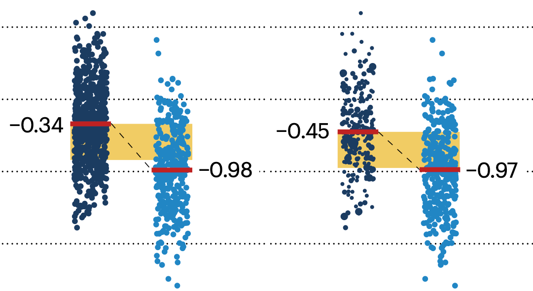
In many experimental designs, we need to keep in mind the possibility of confounding variables, which may give rise to bias in the estimate of the treatment effect.

If the control and experimental groups aren't matched (or, roughly, similar enough), this bias can arise.
Sometimes this can be dealt with by randomizing, which on average can balance this effect out. When randomization is not possible, propensity score matching is an excellent strategy to match control and experimental groups.
Kurz, C.F., Krzywinski, M. & Altman, N. (2024) Points of significance: Propensity score matching. Nat. Methods 21:1770–1772.
Nasa to send our human genome discs to the Moon
We'd like to say a ‘cosmic hello’: mathematics, culture, palaeontology, art and science, and ... human genomes.


Comparing classifier performance with baselines
All animals are equal, but some animals are more equal than others. —George Orwell
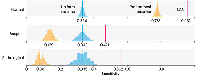
This month, we will illustrate the importance of establishing a baseline performance level.
Baselines are typically generated independently for each dataset using very simple models. Their role is to set the minimum level of acceptable performance and help with comparing relative improvements in performance of other models.

Unfortunately, baselines are often overlooked and, in the presence of a class imbalance, must be established with care.
Megahed, F.M, Chen, Y-J., Jones-Farmer, A., Rigdon, S.E., Krzywinski, M. & Altman, N. (2024) Points of significance: Comparing classifier performance with baselines. Nat. Methods 21:546–548.
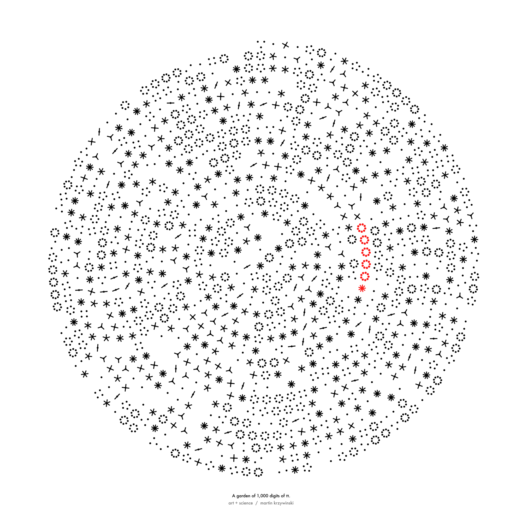
Happy 2024 π Day—
sunflowers ho!
Celebrate π Day (March 14th) and dig into the digit garden. Let's grow something.

How Analyzing Cosmic Nothing Might Explain Everything
Huge empty areas of the universe called voids could help solve the greatest mysteries in the cosmos.
My graphic accompanying How Analyzing Cosmic Nothing Might Explain Everything in the January 2024 issue of Scientific American depicts the entire Universe in a two-page spread — full of nothing.
The graphic uses the latest data from SDSS 12 and is an update to my Superclusters and Voids poster.
Michael Lemonick (editor) explains on the graphic:
“Regions of relatively empty space called cosmic voids are everywhere in the universe, and scientists believe studying their size, shape and spread across the cosmos could help them understand dark matter, dark energy and other big mysteries.
To use voids in this way, astronomers must map these regions in detail—a project that is just beginning.
Shown here are voids discovered by the Sloan Digital Sky Survey (SDSS), along with a selection of 16 previously named voids. Scientists expect voids to be evenly distributed throughout space—the lack of voids in some regions on the globe simply reflects SDSS’s sky coverage.”
voids
Sofia Contarini, Alice Pisani, Nico Hamaus, Federico Marulli Lauro Moscardini & Marco Baldi (2023) Cosmological Constraints from the BOSS DR12 Void Size Function Astrophysical Journal 953:46.
Nico Hamaus, Alice Pisani, Jin-Ah Choi, Guilhem Lavaux, Benjamin D. Wandelt & Jochen Weller (2020) Journal of Cosmology and Astroparticle Physics 2020:023.
Sloan Digital Sky Survey Data Release 12
Alan MacRobert (Sky & Telescope), Paulina Rowicka/Martin Krzywinski (revisions & Microscopium)
Hoffleit & Warren Jr. (1991) The Bright Star Catalog, 5th Revised Edition (Preliminary Version).
H0 = 67.4 km/(Mpc·s), Ωm = 0.315, Ωv = 0.685. Planck collaboration Planck 2018 results. VI. Cosmological parameters (2018).
constellation figures
stars
cosmology
Error in predictor variables
It is the mark of an educated mind to rest satisfied with the degree of precision that the nature of the subject admits and not to seek exactness where only an approximation is possible. —Aristotle
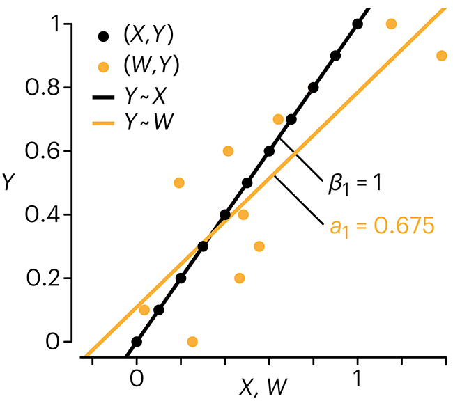
In regression, the predictors are (typically) assumed to have known values that are measured without error.
Practically, however, predictors are often measured with error. This has a profound (but predictable) effect on the estimates of relationships among variables – the so-called “error in variables” problem.

Error in measuring the predictors is often ignored. In this column, we discuss when ignoring this error is harmless and when it can lead to large bias that can leads us to miss important effects.
Altman, N. & Krzywinski, M. (2024) Points of significance: Error in predictor variables. Nat. Methods 21:4–6.
Background reading
Altman, N. & Krzywinski, M. (2015) Points of significance: Simple linear regression. Nat. Methods 12:999–1000.
Lever, J., Krzywinski, M. & Altman, N. (2016) Points of significance: Logistic regression. Nat. Methods 13:541–542 (2016).
Das, K., Krzywinski, M. & Altman, N. (2019) Points of significance: Quantile regression. Nat. Methods 16:451–452.


