Infinity with Max Cooper — In Six Minutes
To Infinity and beyond!
—Buzz Lightyear
contents
The video was created with a custom-made kinetic typography system that emulates a low-fi terminal display. The system is controlled by a plain-text configuration file that defines scenes and timings—there is no GUI. There is also no post-processing of any kind, such as After Effects. Everything that you see in the final video was generated programatically. The code was written over a period of about a month.
This page describes this system's design in detail. Fair warning: it gets into the weeds quite a bit.
The original music score for Aleph 2 is 6 minutes and 34 seconds in length.
The score tempo is 118 bpm (1.967 beats per second, 0.082 beats per frame). There are 194.1 measures in the video (29.5 measures per minute, 0.492 measures per second, 0.020 measures per frame).
The video format is 24 fps, so the track comprises 9,473 frames (1440 frames per minute, 48.814 frames per measure, 12.203 frames per beat, 3.051 frames per 16th note).
The typography uses the Classic Console font, expanded by me to include set theory characters such as `\aleph`, `\mathbb{N}`, `\mathbb{R}`, `\notin`, `\varnothing` and so on.
The video is 16:9 and each frame is rendered at 1,920 × 1,080. Text is set on a grid of 192 columns and 83 rows (maximum of 15,936 characters per frame).
The entire video is first initialized as an `(x,y,z)` matrix of size 192 × 83 × 9,473 (150,961,728 elements). The `z` dimension is the time dimension and each matrix slice, for example `(x,y,1)`, corresponds to the first frame.
The video is then built up from a series of scenes. Briefly, this process is single-threaded and takes about 30 minutes and during this time the matrix is populated with text characters. As the scenes are built up, each element in the matrix stays blank or has a colored character assigned to it. Periodically, effects are added such as random glitches. All elements are synchronized to the tempo of the score and transitions can be triggered from drum score midi files. For example, in parts, the background for each frame flashes to the kick and snare. I get into the detail of this below.
Once the matrix has been fully populated, each frame is output to a PNG file (e.g. 000000.png ... 009472.png). Below you can see 10 frames in the range 2490–2499 from the Bijection 2 section of the video at 1:42.
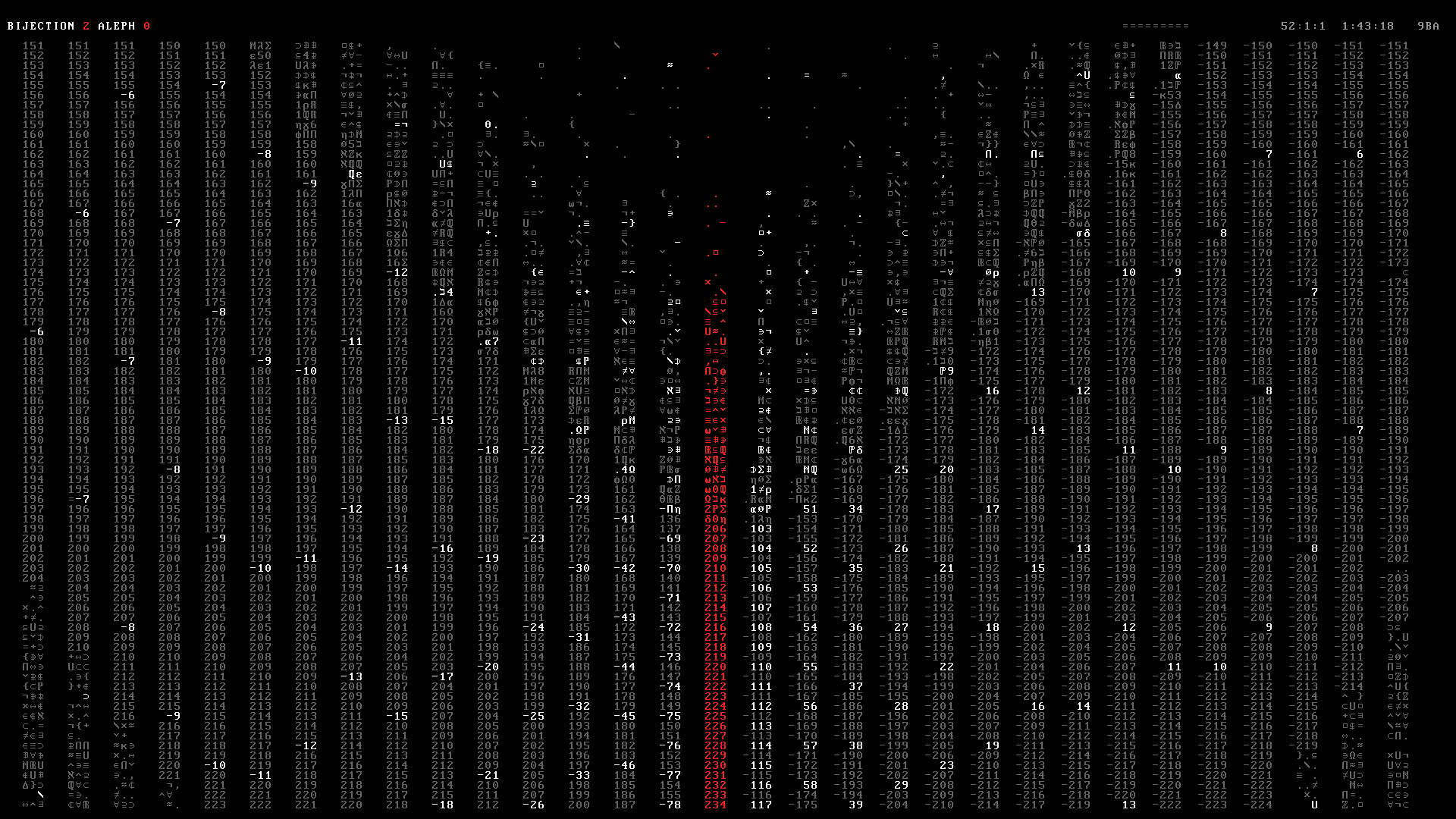
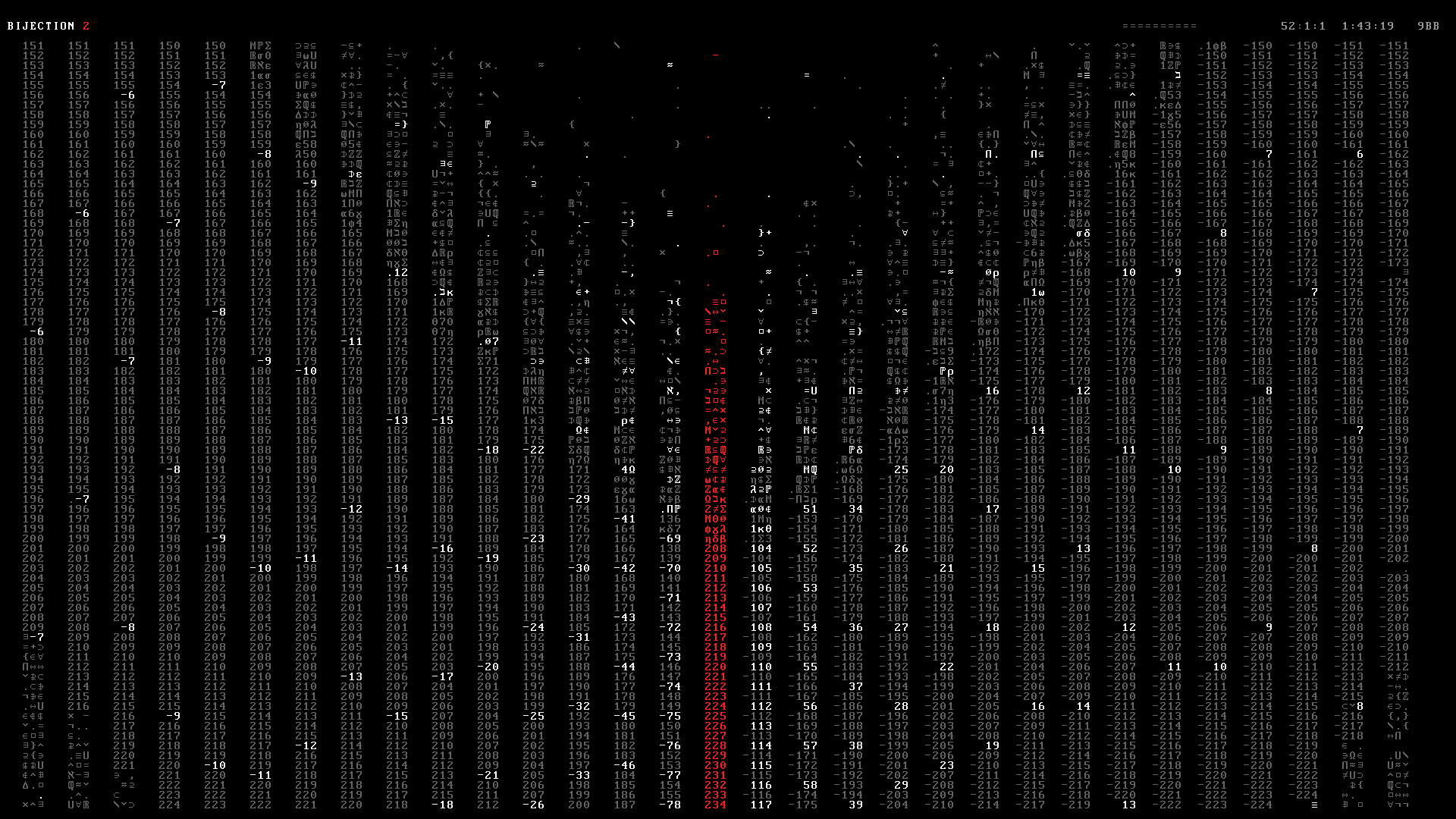
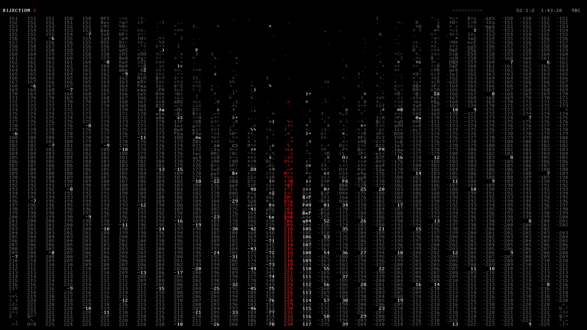
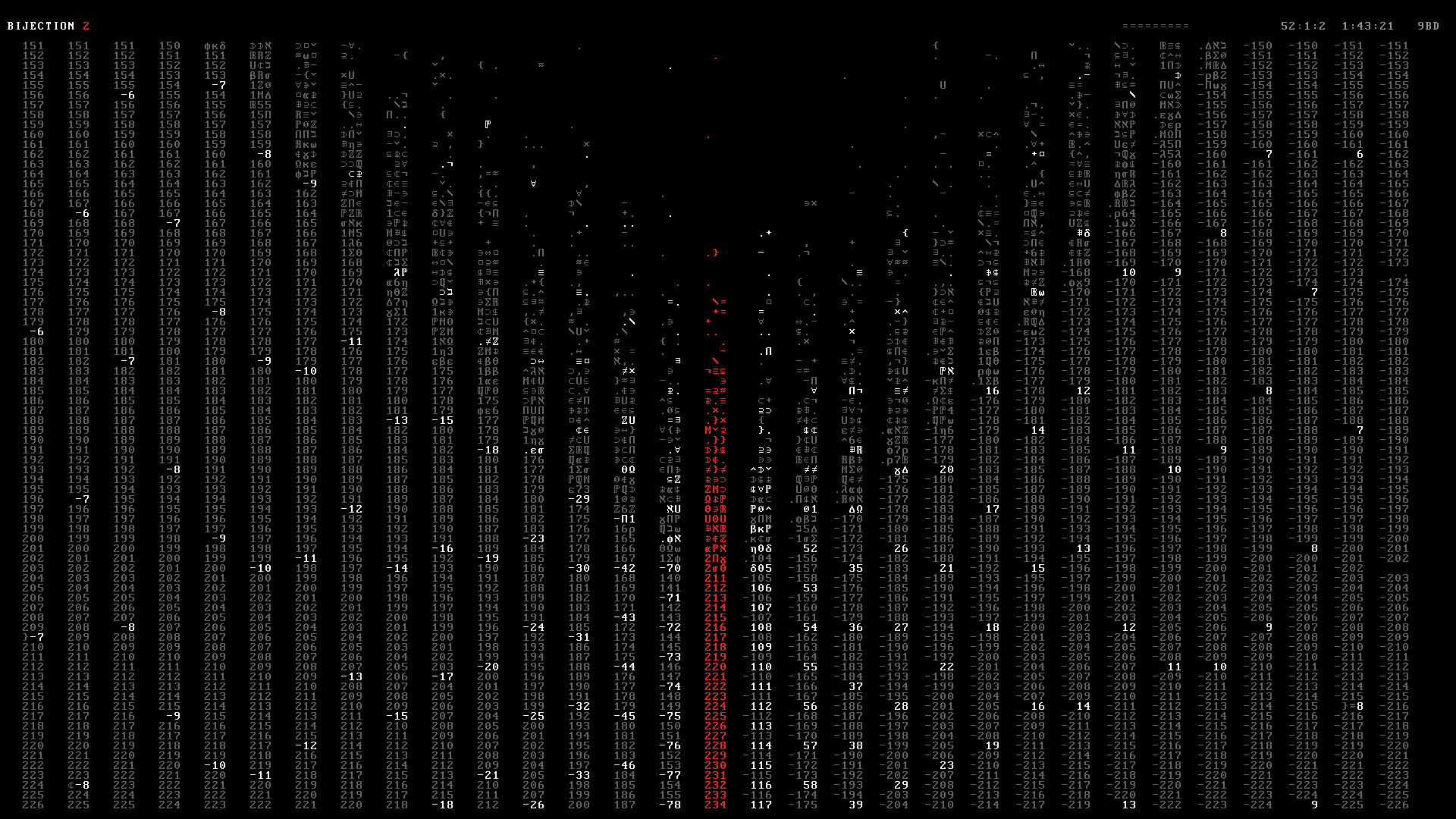
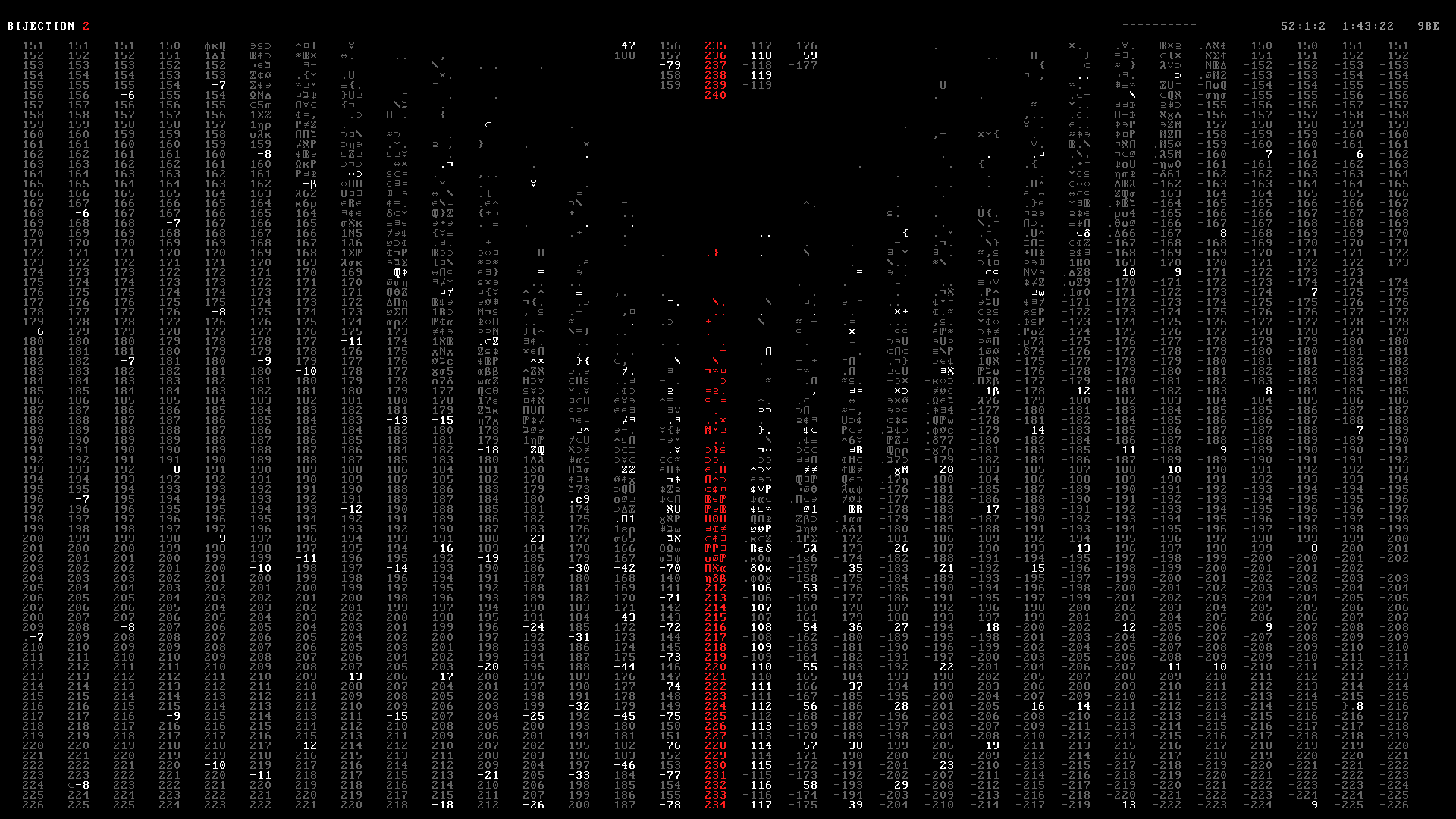
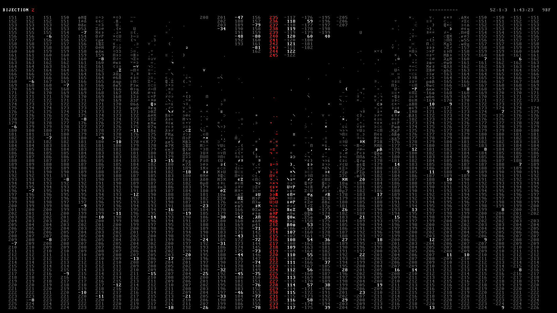
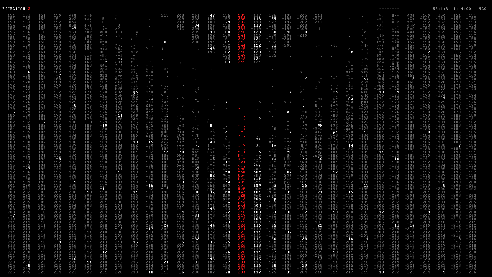
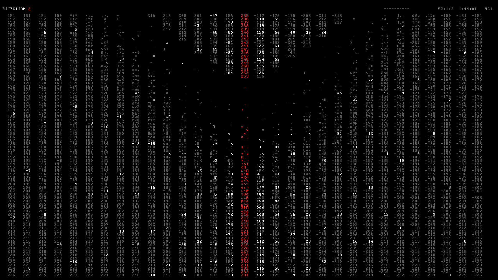
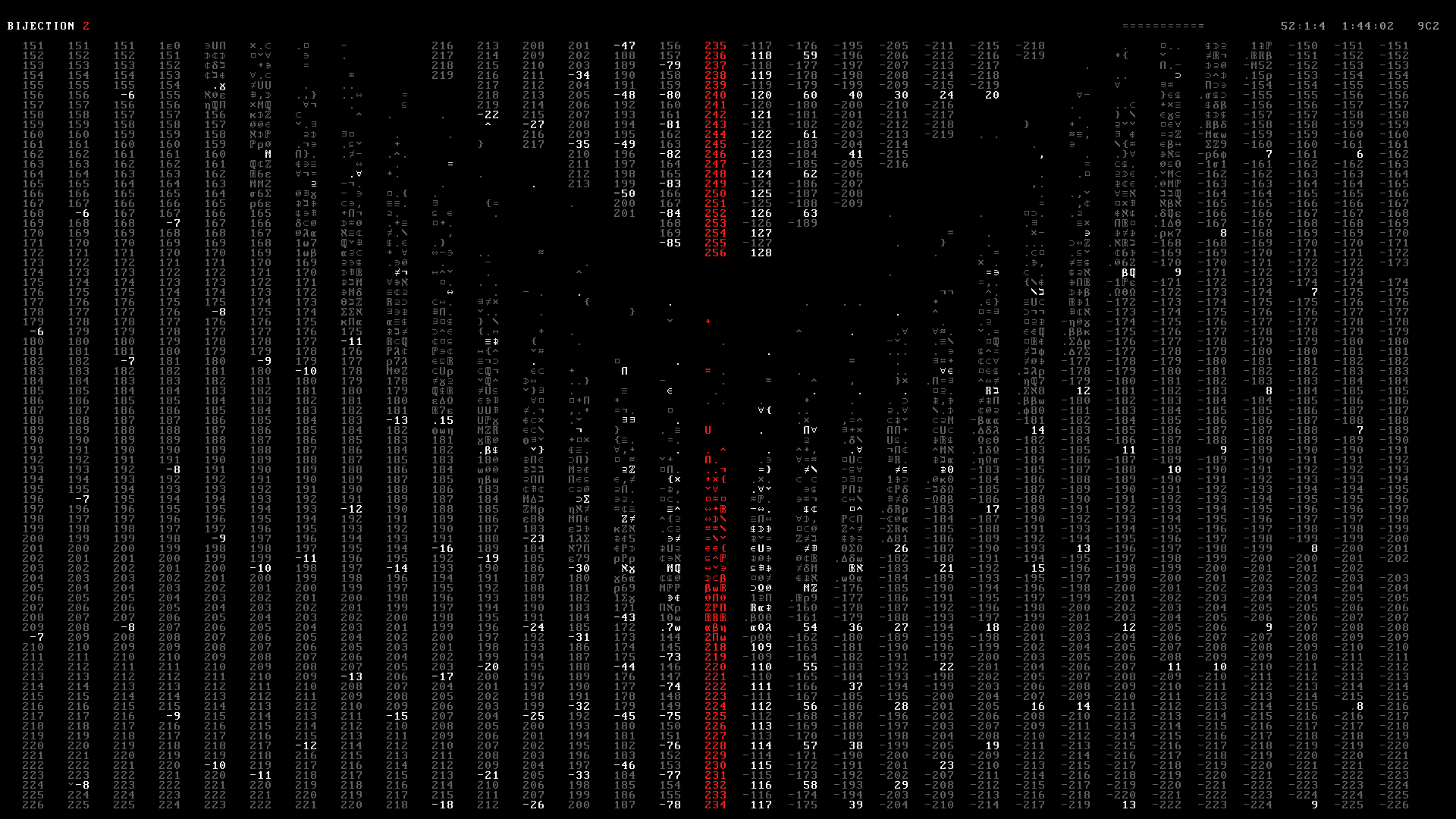
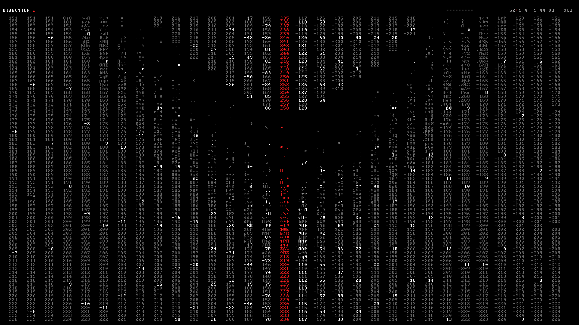
The frames were then stitched into a PNG movie in 24-bit RGB color space using ffmpeg.
ffmpeg -thread_queue_size 32 -r 24 -y -i "frames/aleph/%06d.png" $offset $seek -i wav/aleph.wav -pix_fmt rgb24 -avoid_negative_ts make_zero -shortest -r 24 -c:v png -f mov aleph.mov
The .mov file is then converted into DXV format used by the Resolume VJ software that Max Cooper uses in his shows to control the displays.
If you watch the video on YouTube, please know that the YouTube temporal and chroma compression greatly reduces the quality of the original 24-bit RGB master, which was used for the Barbican Hall performance. The YouTube compression bleaches out the vibrant red, which really pops out in the master version, and blurs frames during fast strobing, which neuters parts of the video that are designed to be overwhelming, such as the drop transition to 24 fps strobing during the natural number power set.
Here is Max's original direction for the video's narrative and art style.
I want to show ever growing lists of numbers, then split the lists somehow (left/right of screen) and show how you can pair subsets of Aleph 0 / integers with themselves, then show how Cantor's diagonal argument can be used to pair the fractions with the natural numbers, then show his other diagonal argument for proving the reals are greater than Aleph 0, then show the process (very roughly and with maximum artistic licence if necessary) of taking the power set of infinite sets to create larger infinities to get up to Aleph 1, Aleph 2, and maybe further if the system allows. In the end it should just be complete text/number chaos on screen along with the intense chaos of the audio.
We'd have to be very careful to avoid any Matrix reference visually! ... but that low-fi / command line style would be suitable I think.
In terms of animation, the technical requirements were relatively simple. Everything would be rendered with a fixed-width font with no anti-aliasing and the color palette would be very limited (e.g. black, grey, white and a red for emphasis). Nothing other than characters would be drawn (no lines, circles or other geometrical shapes) and there would be no gradients. Basically, very lo-fi and 8-bit.
Despite the fact that I've never made any kind of animation before, I thought that these requirements could be relatively easy to achieve. After all, if worse came to worst, I told myself that I could always generate the video frame-by-frame.
However, it quickly became obvious that traditional keyframe systems could not be easily used to tell our story. Tools like Adobe After effects rely on interpolation between keyframes. But in our video every frame is essentially a keyframe. This meant that any kind of interpolation between scene points would have to be programmed—while After Effects makes it easy to move things around on the screen, it requires scripting to generate content based on lists of numbers, set elements, and so on. And since I have no experience in After Effects, I thought it would be faster to code my own system than to learn After Effects' expression language to (possibly) later discover that what I wanted to do was either hard or practically impossible for me to achieve within our time frame (a month).
I knew that I was reasonably good at prototyping and generating custom visualizations, so it felt safer to create something from scratch.
The final version of the system, which is very much a prototype, is about 6,000 lines of Perl. The Aleph 2 video is built out from about 2,000 lines of plain-text configuration that defines scenes, timings and effects.
It took about a week to figure out how to design the system. As we were building out the video, I iterated between creating the story and creating the system to tell the story. This was iterative and felt very much like trying to simultaneously building and flying a plane.
At times, the entire process would crash down on me because some tiny tweak fundamentally changed how everything worked.
For example, one extremely nagging aspect of the code that I patched only half-way through the entire process had to do with how time was specified. From the start, I made use of measure:beat:16note notation, such as for scene starts and ends (e.g. 2:2 to 4:1 meant a scene started on measure 2 beat 2 and stopped at measure 4 beat 1).
This notation used 1-indexing (e.g. 1:1:1 is the first 16th note of the score). 0-indexing would have been unintuitive because musically one counts beats as 1, 2, 3, 4 and not 0, 1, 2, 3. Importantly, I wanted the way we referred to timings in conversation (e.g. on the "and of 2" of the 4th measure) to be directly reflected in the code.
All this made sense until I needed a notation to express duration. When I started using 1:1 to indicate a duration of 1 measure and 1 beat, I had to reconcile the difference between 1:1 as a point in time and as a duration—the former specified the beginning of the interval (e.g. frame=0) and the latter the end (frame=61). It also took me forever to decide whether the duration of 5 beats should be expressed as 1:2 (e.g. end is start of beat 2) or 1:1 (e.g. end is end of beat 1).
The fact that the video frame rate is 24 fps made things even more complicated. At this frame rate, there are 3.051 frames per 16th note. This meant that any duration of 1 frame (which happens during fast strobing) couldn't be expressed by the integer notation of measure:note:16note. I didn't want to have to write 0:0:0.3278, which seemed a tedious way of saying "1 frame". Furthermore, because frames didn't neatly match up to 16th note boundaries, quite a lot of time is spent checking that timing definitions don't suffer from rounding issues.
In the final video, you'll see the measure timer in the upper right corner. The : between the measure and beat flashes as a red + on the beat (118 bpm). Next to the measure timestamp you'll see a min:sec:frame timestamp and hexadecimal readout of the frame number.
The video is composed of a series of scenes, each with a specific start and end time, as well as other parameters. The start and end of scenes was typically informed by changes in the music, such as breaks.
A scene is a short clip of the video in which similar content is being shown. For example, at the start where we count the natural numbers, each filling scene is a scene. Below are the timing definitions for the first three screens of natural counts.
<scene>
name       = nc1
timing     = count1
ease       = 0.6
ease_step  = 0
start      = 4m     # starts at measure 4
len        = 13m    # lasts for 13 measures
k_start    = 1      # start counting at 1
</scene>

<scene>
name       = nc2
timing     = nc_timing
ease       = 0.8
start      = 17m    # starts at measure 17
len        = 6m     # lasts for 6 measures
</scene>

<scene>
name       = nc3
timing     = nc_timing
ease       = 0.7
start      = 23m
len        = 2m
</scene>
For each scene, I generate the numbers that will appear in the scene and then distribute their time of appearance across the duration of the scene, subject to some easing.
Some scenes are more complicated and consist of several screens worth of content. Once the screen is filled, it's cleared and then more content is shown. For example, in the bijection section the natural numbers down the center take 2 measures to fill at first but next time the fill takes less time at 2 * 0.8 measures. We keep multiplying the fill time by 0.8 until we reach a minimum of 6 frames.
<timing bijection-n>
time_to_fill_start = 2m
time_to_fill_mult  = 0.8
time_to_fill_end   = 6
time_pause_start   = 2
time_blank_start   = 2
</timing>
A lot of the effects appear as set theory characters that display on the screen briefly in sync with the music.
Through the video, there are a lot of transitions and fades that look like text is decaying.
For example, a 9 might decay into an 8 then a 7 and all the way down to 0 and then be wiped from the screen. At other times, a 9 might decay by randomly selecting the next character from a set of lists, such as
["@","#","\$","%","&","*"]
["[","]","{","}","<",">"]
[";",":","-","+","="]
[".",","]
So a 9 might decay as 9%]+ across some number of frames, depending on whether the decay is fast or slow.
The timing and speed of this decay process took a long time to tweak. There are many parts in the video where the decay speeds up, or slows down and many times the decay is triggered by percussion. For example, the snare can be made to initiate some characters on the screen to rapidly decay.
The decay is processed as an effect after the basic scene is laid out. During this process, we can look ahead in time to know what is coming at a given screen position and terminate the decay if, for example, a new character appears. Alternatively, the decay can bleed into the next scene, if the rate at which it happens is slow and crosses scene boundaries.
Percussion, particularly the snare, are used to trigger characters to flash and decay.
For example, between measures 52 and 65, we flash one of the characters from the set braces = {, }. The braces appear only where characters are already on the screen (writeonchar = 1) with a probability of flash_rate = 0.1 at any given character position.
Immediately upon being drawn, these braces decay (see below) into the list of characters defined by decay_set = setrapid.
<scene>
name        = snare
action      = midi_trigger
position    = full_screen
midi_sets   = snare
midi_action = cascade_red_star_subtle
start       = 52m
end         = 65m
</scene>

<midi_action cascade_red_braces_subtle>
action = char_flash(flash_char_set=>"braces",writeonchar=>1,
                    rgb=>"red",flash_rate=>0.1,
                    decay_rate=>1,decay_delay=>0,
                    decay_punch=>0,decay_set=>"setrapid")
</midi_action>
Because the drum component of the video was a live studio recording, I generated a midi file for the percussions by demarcating the wave form of their sound. This transcription process took a while and care had to be taken to identify the instruments correctly (e.g. snare vs rim shot) to have a list of events that matched the volume.
Once I had a list of all the percussion events, I could create effects that would appear to coincide with these times. For example, every time a snare was hit an effect could trigger 50% of the time.
By far, the bulk of the time in making this video was spent on tweaking the density, duration and decay of effects. Towards the end, between measures 160 and 167, when powersets of naturals and reals are being shown many effects are stacked. For example, the kick drum is used to decay and fade the natural powersets on the left of the screen while the snare does the same for the real powersets on the right.
In modern animation systems you would have an interface that could help in defining timings and effect curves, because my system is controlled by plain text inputs, of the kind that you see above, each set of effects was lovingly tuned by hand by adjusting measure starts and ends and rates in the configuration file.
These configuration files got to be quite long. For example, here are the
scene definitions (storyboard.v3.conf),
effect scenes (effects.conf) and the
midi and decay timings (aleph.conf).
I don't expect that these will make total sense to anyone and post them here to give you more of a flavour of what is happening under the hood.
Beyond Belief Campaign BRCA Art
Fuelled by philanthropy, findings into the workings of BRCA1 and BRCA2 genes have led to groundbreaking research and lifesaving innovations to care for families facing cancer.
This set of 100 one-of-a-kind prints explore the structure of these genes. Each artwork is unique — if you put them all together, you get the full sequence of the BRCA1 and BRCA2 proteins.
Propensity score weighting
The needs of the many outweigh the needs of the few. —Mr. Spock (Star Trek II)
This month, we explore a related and powerful technique to address bias: propensity score weighting (PSW), which applies weights to each subject instead of matching (or discarding) them.
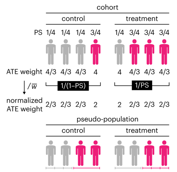
Kurz, C.F., Krzywinski, M. & Altman, N. (2025) Points of significance: Propensity score weighting. Nat. Methods 22:1–3.
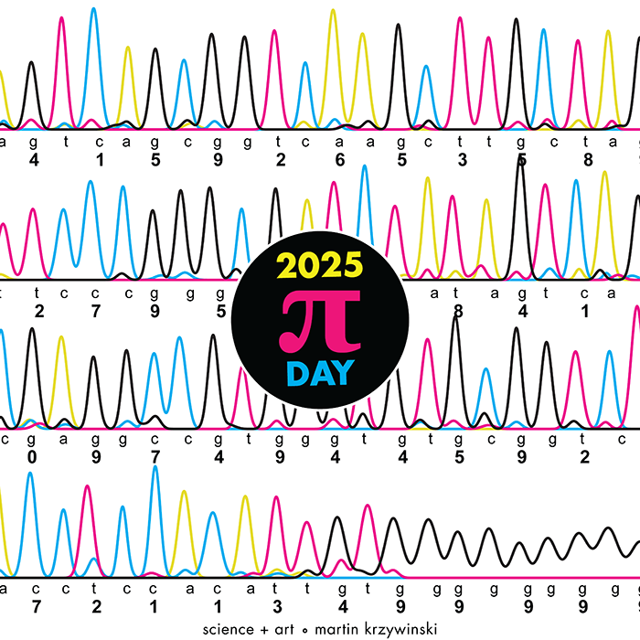
Happy 2025 π Day—
TTCAGT: a sequence of digits
Celebrate π Day (March 14th) and sequence digits like its 1999. Let's call some peaks.
Crafting 10 Years of Statistics Explanations: Points of Significance
I don’t have good luck in the match points. —Rafael Nadal, Spanish tennis player
Points of Significance is an ongoing series of short articles about statistics in Nature Methods that started in 2013. Its aim is to provide clear explanations of essential concepts in statistics for a nonspecialist audience. The articles favor heuristic explanations and make extensive use of simulated examples and graphical explanations, while maintaining mathematical rigor.
Topics range from basic, but often misunderstood, such as uncertainty and P-values, to relatively advanced, but often neglected, such as the error-in-variables problem and the curse of dimensionality. More recent articles have focused on timely topics such as modeling of epidemics, machine learning, and neural networks.
In this article, we discuss the evolution of topics and details behind some of the story arcs, our approach to crafting statistical explanations and narratives, and our use of figures and numerical simulations as props for building understanding.
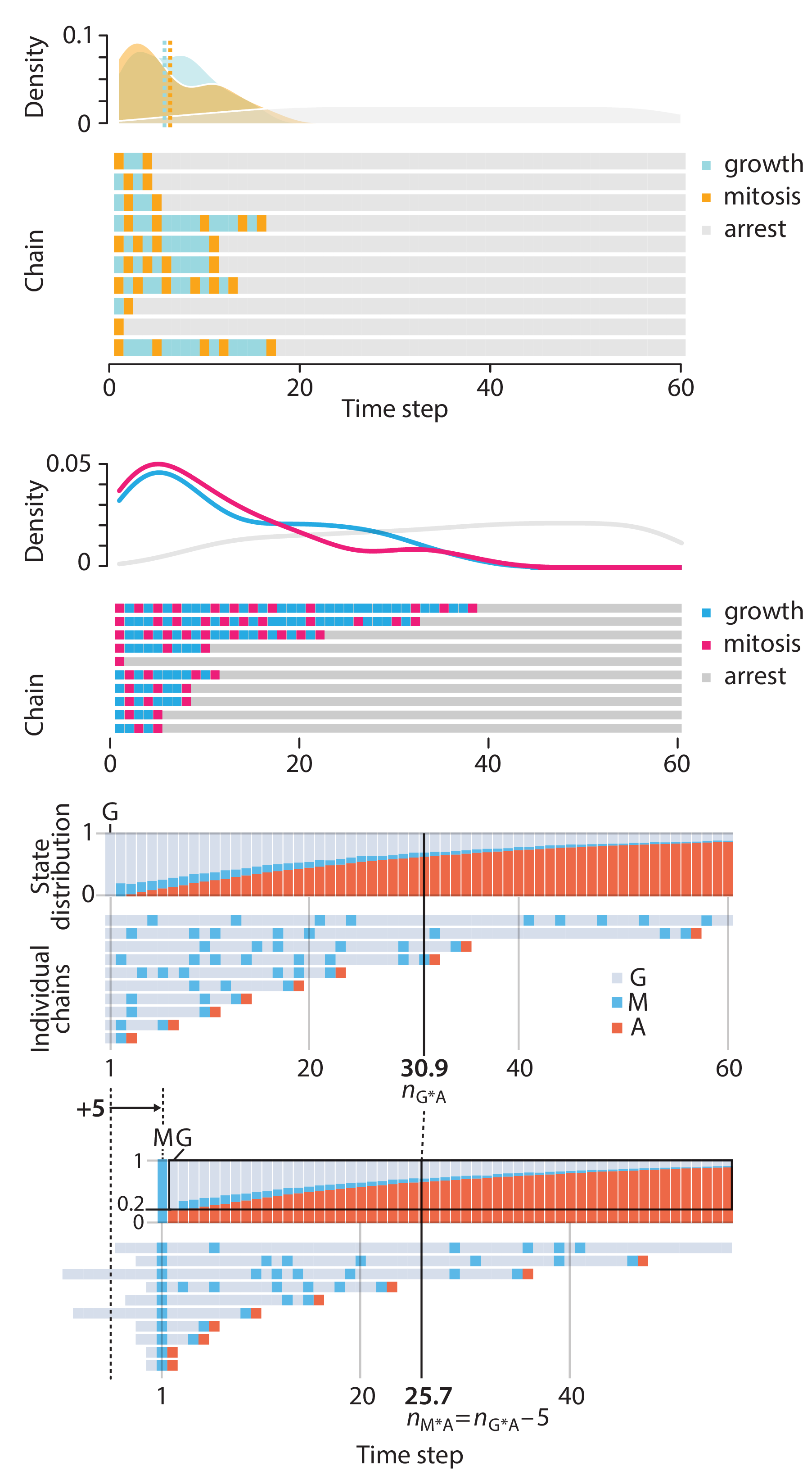
Altman, N. & Krzywinski, M. (2025) Crafting 10 Years of Statistics Explanations: Points of Significance. Annual Review of Statistics and Its Application 12:69–87.
Propensity score matching
I don’t have good luck in the match points. —Rafael Nadal, Spanish tennis player
In many experimental designs, we need to keep in mind the possibility of confounding variables, which may give rise to bias in the estimate of the treatment effect.
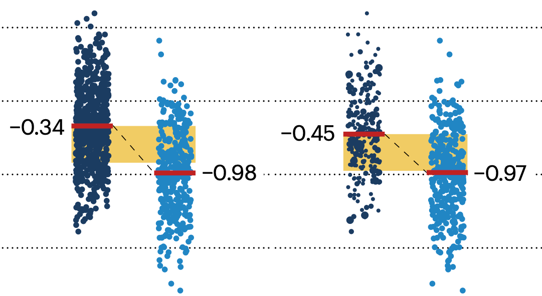
If the control and experimental groups aren't matched (or, roughly, similar enough), this bias can arise.
Sometimes this can be dealt with by randomizing, which on average can balance this effect out. When randomization is not possible, propensity score matching is an excellent strategy to match control and experimental groups.
Kurz, C.F., Krzywinski, M. & Altman, N. (2024) Points of significance: Propensity score matching. Nat. Methods 21:1770–1772.
Understanding p-values and significance
P-values combined with estimates of effect size are used to assess the importance of experimental results. However, their interpretation can be invalidated by selection bias when testing multiple hypotheses, fitting multiple models or even informally selecting results that seem interesting after observing the data.
We offer an introduction to principled uses of p-values (targeted at the non-specialist) and identify questionable practices to be avoided.
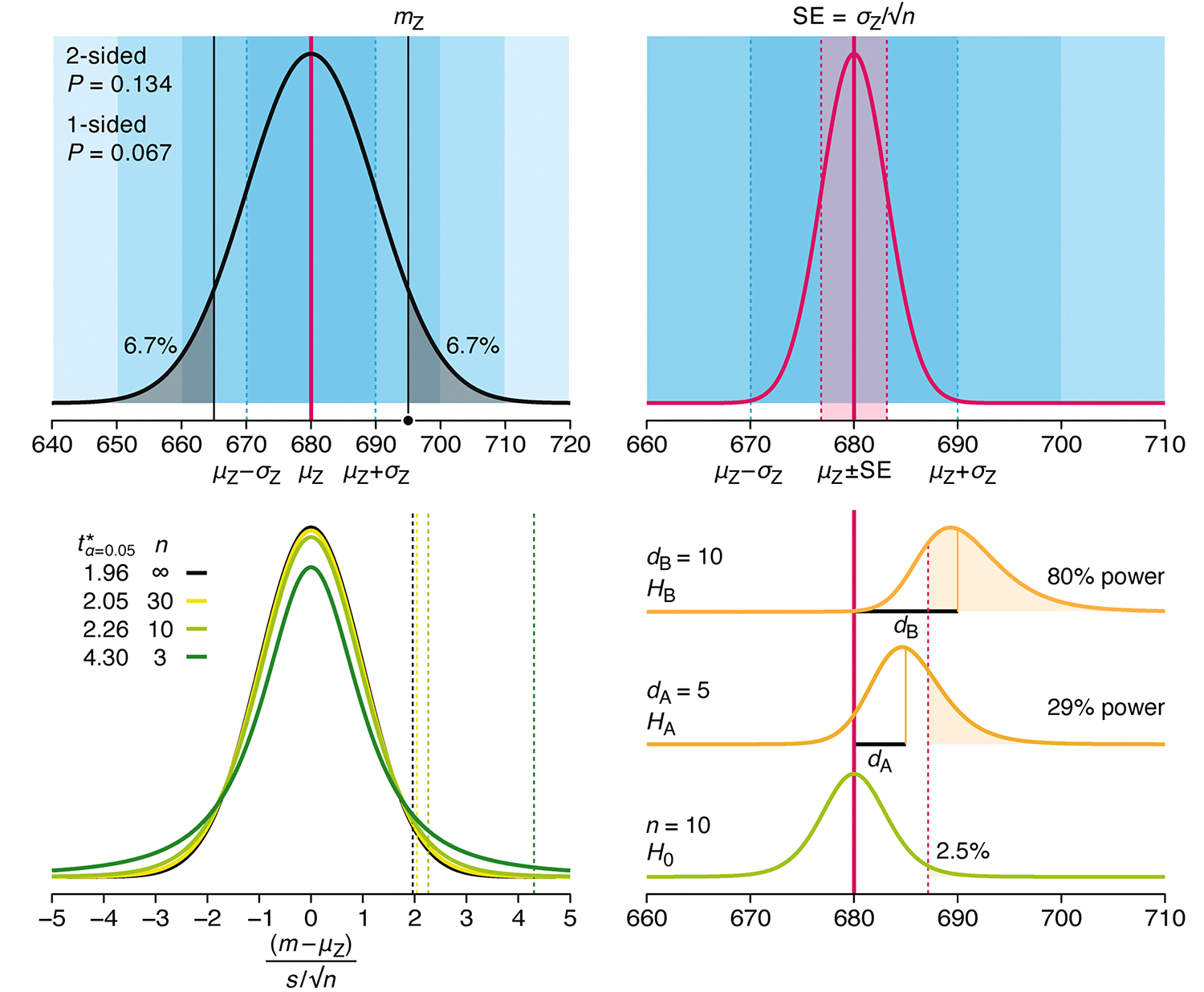
Altman, N. & Krzywinski, M. (2024) Understanding p-values and significance. Laboratory Animals 58:443–446.
